5️⃣ Mujoco
Learning Objectives
- Understand how PPO can be used to train agents in continuous action spaces
- Install and interact with the MuJoCo physics engine
- Train an agent to solve the Hopper environment
A note for anyone who has fought MuJoCo installs before - the original
mujoco-pyenvironments were notoriously demanding about library versions (and required Python<3.11, breaking Colab). None of that applies here: our MuJoCo section runs on Brax (MuJoCo physics in JAX, on the GPU), which is a plain pip install with no special Python version required.
Installation & Rendering
The physics packages (brax, mujoco, and the pinned jax) were installed along with the rest of the course requirements - the first commented line below is only needed if you're on a fresh machine (e.g. Colab).
Rendering videos is the one part that touches system libraries. We replay rollouts through the official mujoco.Renderer (via the thin wrapper in part3_ppo/mujoco_rendering.py), which produces the classic gym-style MP4s - robot geometry, checkerboard floor, and a track camera that follows the agent. Offscreen rendering needs some OpenGL backend to exist on the machine, and mujoco alone handles this badly on headless boxes (it commits to a backend at import time, defaulting to GLFW which needs a display) - our wrapper instead probes for one that actually works ($MUJOCO_GL if set, otherwise the first of EGL → OSMesa → GLFW). Depending on your machine:
- You have a display (e.g. your own Linux desktop): nothing to do - GLFW will work.
- Headless with sudo (most rented GPU boxes): install OSMesa, a software OpenGL implementation, with the single
apt-getline below. (If your machine has full NVIDIA OpenGL drivers - Colab does - you can instead setos.environ["MUJOCO_GL"] = "egl"before rendering, for GPU-accelerated rendering.) - Headless without sudo (shared clusters): install OSMesa from conda-forge instead, with the
conda createline below. Note the version pin:mesalib25+ no longer ships OSMesa. You don't need to activate the env or setLD_LIBRARY_PATH- our renderer finds and preloadslibOSMesafrom$CONDA_PREFIXor~/.conda/envs/*automatically.
If no OpenGL backend can be set up at all, record_brax_video falls back to Brax's interactive three.js viewer, which renders client-side in your browser with no GL needed - you'll still see your agent, just in an interactive 3D viewer rather than an MP4.
%pip install brax==0.14.2 mujoco "jax[cuda12]==0.10.1"   # only on a fresh machine (e.g. Colab); already in the course requirements

!sudo apt-get install -y libosmesa6                        # headless + sudo: software GL for MP4 rendering
!conda create -y -n oslibs -c conda-forge "mesalib=24.3.4" # headless, no sudo: same library via conda-forge
To test that this works, run the following. The first time you run this, it might take about 1-2 minutes, and throw up several warnings and messages. But the cell should still run without raising an exception, and all subsequent times you run it, it should be a lot faster (with no error messages).
env = BraxEnvs("Hopper-v4", num_envs=1, seed=0)  # GPU (Brax) Hopper

print(env.single_action_space)
print(env.single_observation_space)
Box(-1.0, 1.0, (3,), float32)
Box(-inf, inf, (11,), float32)
Previously, we've dealt with discrete action spaces (e.g. going right or left in Cartpole). But here, we have a continuous action space - the actions take the form of a vector of 3 values, each in the range [-1.0, 1.0].
Question - after reading the documentation page, can you see exactly what our 3 actions mean?
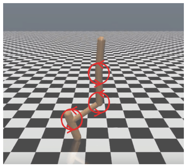
They represent the torque applied between the three different links of the hopper. There is:
- The thigh rotor (i.e. connecting the upper and middle parts of the leg),
- The leg rotor (i.e. connecting the middle and lower parts of the leg),
- The foot rotor (i.e. connecting the lower part of the leg to the foot).
How do we deal with a continuous action space, when it comes to choosing actions? Rather than our actor network's output being a vector of logits which we turn into a probability distribution via Categorical(logits=logits), we instead have our actor output two vectors mu and log_sigma, which we turn into a normal distribution which is then sampled from.
The observations take the form of a vector of 11 values describing the position, velocity, and forces applied to the joints. So unlike for Atari, we can't directly visualize the environment from its observations. Instead, record_brax_video replays a recorded rollout through mujoco.Renderer (via part3_ppo/mujoco_rendering.py, which handles headless GL-backend selection), giving the same video gym's env.render() would: the actual robot geometry on a checkerboard floor, with a tracking camera that follows the agent. This needs an OpenGL backend (see "Installation & Rendering" above); if none is available it falls back to Brax's interactive in-browser 3D viewer. The cell below shows a short random rollout of an untrained Hopper (it just topples over):
env = BraxEnvs("Hopper-v4", num_envs=1, seed=0)
# Render a short *random* rollout to a gym-style MP4 (tracking camera; falls back to Brax's
# in-browser 3D viewer if no OpenGL backend is available).
display(record_brax_video(env, actor=None, steps=150))
And here's what a trained Hopper looks like (a learned hopping gait, replayed in the interactive player):
Implementational details of MuJoCo
Clipping, Scaling & Normalization (details #5-9)
Just like for Atari, there are a few messy implementational details which will be taken care of with gym wrappers. For example, if we generate our actions by sampling from a normal distribution, then there's some non-zero chance that our action will be outside of the allowed action space. We deal with this by clipping the actions to be within the allowed range (in this case between -1 and 1).
See the function prepare_mujoco_env within part3_ppo/utils (and read details 5-9 on the PPO page) for more information.
Actor and Critic networks (details #1-4)
Our actor and critic networks are quite similar to the ones we used for cartpole. They won't have shared architecture.
Question - can you see why it's less useful to have shared architecture in this case, relative to the case of Atari?
The point of the shared architecture in Atari was that it allowed our critic and actor to perform feature extraction, i.e. the early part of the network (which was fed the raw pixel input) generated a high-level representation of the state, which was then fed into the actor and critic heads. But for CartPole and for MuJoCo, we have a very small observation space (4 discrete values in the case of CartPole, 11 for the Hopper in MuJoCo), so there's no feature extraction necessary.
The only difference will be in the actor network. There will be an actor_mu and actor_log_sigma network. The actor_mu will have exactly the same architecture as the CartPole actor network, and it will output a vector used as the mean of our normal distribution. The actor_log_sigma network will just be a bias, since the standard deviation is state-independent (detail #2).
Because of this extra complexity, we'll create a class for our actor and critic networks.
Exercise - implement Actor and Critic
As discussed, the architecture of actor_mu is identical to your cartpole actor network, and the critic is identical. The only difference is the addition of actor_log_sigma, which you should initialize as an nn.Parameter object of shape (1, num_actions).
Your Actor class's forward function should return a tuple of (mu, sigma, dist), where mu and sigma are the parameters of the normal distribution, and dist was created from these values using torch.distributions.Normal.
Why do we use log_sigma rather than just outputting sigma ?
We have our network output log_sigma rather than sigma because the standard deviation is always positive. If we learn the log standard deviation rather than the standard deviation, then we can treat it just like a regular learned weight.
Tip - when creating your distribution, you can use the broadcast_to tensor method, so that your standard deviation and mean are the same shape.
We've given you the function get_actor_and_critic_mujoco (which is called when you call get_actor_and_critic with mode="mujoco"). All you need to do is fill in the Actor and Critic classes.
class Critic(nn.Module):
    def __init__(self, num_obs):
        super().__init__()
        raise NotImplementedError()

    def forward(self, obs) -> Tensor:
        raise NotImplementedError()


class Actor(nn.Module):
    actor_mu: nn.Sequential
    actor_log_sigma: nn.Parameter

    def __init__(self, num_obs, num_actions):
        super().__init__()
        raise NotImplementedError()

    def forward(self, obs) -> tuple[Tensor, Tensor, t.distributions.Normal]:
        raise NotImplementedError()


def get_actor_and_critic_mujoco(num_obs: int, num_actions: int):
    """
    Returns (actor, critic) in the "classic-control" case, according to description above.
    """
    return Actor(num_obs, num_actions), Critic(num_obs)


tests.test_get_actor_and_critic(get_actor_and_critic, mode="mujoco")
Solution
class Critic(nn.Module):
    def __init__(self, num_obs):
        super().__init__()
        self.critic = nn.Sequential(
            layer_init(nn.Linear(num_obs, 64)),
            nn.Tanh(),
            layer_init(nn.Linear(64, 64)),
            nn.Tanh(),
            layer_init(nn.Linear(64, 1), std=1.0),
        )

    def forward(self, obs) -> Tensor:
        value = self.critic(obs)
        return value


class Actor(nn.Module):
    actor_mu: nn.Sequential
    actor_log_sigma: nn.Parameter

    def __init__(self, num_obs, num_actions):
        super().__init__()
        self.actor_mu = nn.Sequential(
            layer_init(nn.Linear(num_obs, 64)),
            nn.Tanh(),
            layer_init(nn.Linear(64, 64)),
            nn.Tanh(),
            layer_init(nn.Linear(64, num_actions), std=0.01),
        )
        self.actor_log_sigma = nn.Parameter(t.zeros(1, num_actions))

    def forward(self, obs) -> tuple[Tensor, Tensor, t.distributions.Normal]:
        mu = self.actor_mu(obs)
        sigma = t.exp(self.actor_log_sigma).broadcast_to(mu.shape)
        dist = t.distributions.Normal(mu, sigma)
        return mu, sigma, dist
Exercise - additional rewrites
There are a few more rewrites you'll need for continuous action spaces, which is why we recommend that you create a new solutions file for this part (like we've done with solutions.py and solutions_cts.py).
You'll need to make the following changes:
Logprobs and entropy
Rather than probs = Categorical(logits=logits) as your distribution (which you sample from & pass into your loss functions), you'll just use dist as your distribution. Methods like .logprobs(action) and .entropy() will work on dist just like they did on probs.
Note that these two methods will return objects of shape (batch_size, action_shape) (e.g. for Hopper the last dimension will be 3). We treat the action components as independent (detail #4), meaning we take a product of the probabilities, so we sum the logprobs / entropies. For example:
So you'll need to sum logprobs and entropy over the last dimension. The logprobs value that you add to the replay memory should be summed over (because you don't need the individual logprobs, you only need the logprob of the action as a whole).
Logging
You should log mu and sigma during the learning phase.
Below, we've given you a template for all the things you'll need to change (with new class & function names so they don't overwrite the previous versions).
class PPOAgentCts(PPOAgent):
    def play_step(self) -> list[dict]:
        """
        Changes required:
            - actor returns (mu, sigma, dist), with dist used to sample actions
            - logprobs need to be summed over action space
        """
        raise NotImplementedError()


def calc_clipped_surrogate_objective_cts(
    dist: t.distributions.Normal,
    mb_action: Int[Tensor, " minibatch_size *action_shape"],
    mb_advantages: Float[Tensor, " minibatch_size"],
    mb_logprobs: Float[Tensor, " minibatch_size"],
    clip_coef: float,
    eps: float = 1e-8,
) -> Float[Tensor, ""]:
    """
    Changes required:
        - logprobs need to be summed over action space
    """
    assert (mb_action.shape[0],) == mb_advantages.shape == mb_logprobs.shape

    raise NotImplementedError()


def calc_entropy_bonus_cts(dist: t.distributions.Normal, ent_coef: float):
    """
    Changes required:
        - entropy needs to be summed over action space before taking mean
    """
    raise NotImplementedError()


class PPOTrainerCts(PPOTrainer):
    def __init__(self, args: PPOArgs):
        super().__init__(args)
        self.agent = PPOAgentCts(self.envs, self.actor, self.critic, self.memory)

    def compute_ppo_objective(self, minibatch: ReplayMinibatch) -> Float[Tensor, ""]:
        """
        Changes required:
            - actor returns (mu, sigma, dist), with dist used for loss functions (rather than
                getting dist from logits)
            - objective function calculated using new `_cts` functions defined above
            - newlogprob (for logging) needs to be summed over action space
            - mu and sigma should be logged
        """
        raise NotImplementedError()
Solution
class PPOAgentCts(PPOAgent):
    def play_step(self) -> list[dict]:
        """
        Changes required:
            - actor returns (mu, sigma, dist), with dist used to sample actions
            - logprobs need to be summed over action space
        """
        obs = self.next_obs
        terminated = self.next_terminated

        with t.inference_mode():
            # DISCRETE VERSION: derive distribution from the logits
            # dist = Categorical(logits=self.actor(obs))
            # CONTINUOUS VERSION: return distribution object directly
            _, _, dist = self.actor.forward(obs)

        actions = dist.sample()

        # Step the GPU env with the action tensor directly (Brax / swing-up stay on-device)
        next_obs, rewards, next_terminated, next_truncated, infos = self.envs.step(actions)

        # DISCRETE VERSION: no need to sum logprobs
        # logprobs = dist.log_prob(actions)
        # CONTINUOUS VERSION: logprobs need to be summed over action space
        logprobs = dist.log_prob(actions).sum(-1)

        with t.inference_mode():
            values = self.critic(obs).flatten()
        self.memory.add(obs, actions, logprobs, values, rewards, terminated)

        self.next_obs = next_obs
        self.next_terminated = next_terminated.float()

        self.step += self.envs.num_envs
        return infos


def calc_clipped_surrogate_objective_cts(
    dist: t.distributions.Normal,
    mb_action: Int[Tensor, " minibatch_size *action_shape"],
    mb_advantages: Float[Tensor, " minibatch_size"],
    mb_logprobs: Float[Tensor, " minibatch_size"],
    clip_coef: float,
    eps: float = 1e-8,
) -> Float[Tensor, ""]:
    """
    Changes required:
        - logprobs need to be summed over action space
    """
    assert (mb_action.shape[0],) == mb_advantages.shape == mb_logprobs.shape

    # DISCRETE VERSION: no need to sum logprobs
    # logits_diff = probs.log_prob(mb_action) - mb_logprobs
    # CONTINUOUS VERSION: logprobs need to be summed over action space
    logits_diff = dist.log_prob(mb_action).sum(-1) - mb_logprobs

    r_theta = t.exp(logits_diff)

    mb_advantages = (mb_advantages - mb_advantages.mean()) / (mb_advantages.std() + eps)

    non_clipped = r_theta * mb_advantages
    clipped = t.clip(r_theta, 1 - clip_coef, 1 + clip_coef) * mb_advantages

    return t.minimum(non_clipped, clipped).mean()


def calc_entropy_bonus_cts(dist: t.distributions.Normal, ent_coef: float):
    """
    Changes required:
        - entropy needs to be summed over action space before taking mean
    """
    # DISCRETE VERSION: no need to sum entropy
    # return ent_coef * dist.entropy().mean()
    # CONTINUOUS VERSION: entropy needs to be summed over action space
    return ent_coef * dist.entropy().sum(-1).mean()


class PPOTrainerCts(PPOTrainer):
    def __init__(self, args: PPOArgs):
        super().__init__(args)
        self.agent = PPOAgentCts(self.envs, self.actor, self.critic, self.memory)

    def compute_ppo_objective(self, minibatch: ReplayMinibatch) -> Float[Tensor, ""]:
        """
        Changes required:
            - actor returns (mu, sigma, dist), with dist used for loss functions (rather than
                getting dist from logits)
            - objective function calculated using new `_cts` functions defined above
            - newlogprob (for logging) needs to be summed over action space
            - mu and sigma should be logged
        """
        # DISCRETE VERSION: actor returns logits, and we derive dist from them
        # dist = Categorical(logits=self.actor(minibatch.obs))
        # CONTINUOUS VERSION: actor returns distribution object directly
        mu, sigma, dist = self.agent.actor(minibatch.obs)

        values = self.agent.critic(minibatch.obs).squeeze()

        clipped_surrogate_objective = calc_clipped_surrogate_objective_cts(
            dist, minibatch.actions, minibatch.advantages, minibatch.logprobs, self.args.clip_coef
        )
        value_loss = calc_value_function_loss(values, minibatch.returns, self.args.vf_coef)
        entropy_bonus = calc_entropy_bonus_cts(dist, self.args.ent_coef)
        total_objective_function = clipped_surrogate_objective - value_loss + entropy_bonus

        with t.inference_mode():
            # DISCRETE VERSION: no need to sum logprobs
            # newlogprob = dist.log_prob(minibatch.actions)
            # CONTINUOUS VERSION: logprobs need to be summed over action space
            newlogprob = dist.log_prob(minibatch.actions).sum(-1)
            logratio = newlogprob - minibatch.logprobs
            ratio = logratio.exp()
            approx_kl = (ratio - 1 - logratio).mean().item()
            clipfracs = [((ratio - 1.0).abs() > self.args.clip_coef).float().mean().item()]
        # Stash the latest loss components (incl. the policy's mu/sigma) for the progress bar + wandb.
        self.last_metrics = dict(
            value_loss=value_loss.item(),
            clip_surr=clipped_surrogate_objective.item(),
            entropy=entropy_bonus.item(),
            approx_kl=approx_kl,
            mu=mu.mean().item(),
            sigma=sigma.mean().item(),
        )
        if self.args.use_wandb:
            wandb.log(
                dict(
                    total_steps=self.agent.step,
                    values=values.mean().item(),
                    lr=self.scheduler.optimizer.param_groups[0]["lr"],
                    clipfrac=np.mean(clipfracs),
                    **self.last_metrics,
                ),
                step=self.agent.step,
            )

        return total_objective_function
Training MuJoCo
Now, you should be ready to run your training loop! We recommend using the following parameters, to match the original implmentation which the 37 Implementational Details post is based on (but you can experiment with different values if you like).
if SLOW:
    args = PPOArgs(
        env_id="Hopper-v4",
        wandb_project_name="PPOMuJoCo",
        mode="mujoco",
        total_timesteps=8_000_000,
        num_envs=2048,
        num_steps_per_rollout=32,
        num_minibatches=8,
        lr=1e-3,
        gamma=0.97,
        ent_coef=0.0,
        vf_coef=0.5,
    )
    trainer = PPOTrainerCts(args)
    trainer.train()
    # gym-style MP4 of the trained agent (tracking camera; in-browser viewer fallback)
    display(record_brax_video(trainer.envs, trainer.agent.actor))
And Humanoid — a much higher-dimensional body. With the accelerated environment provided by Brax on the GPU the model learns an awkward walking gait in only a few minutes:
if SLOW:
    args = PPOArgs(
        env_id="Humanoid-v4",
        wandb_project_name="PPOMuJoCo",
        mode="mujoco",
        total_timesteps=15_000_000,
        num_envs=2048,
        num_steps_per_rollout=32,
        num_minibatches=8,
        lr=1e-3,
        ent_coef=0.0,
        vf_coef=0.5,
    )
    trainer = PPOTrainerCts(args)
    trainer.train()
    display(record_brax_video(trainer.envs, trainer.agent.actor))
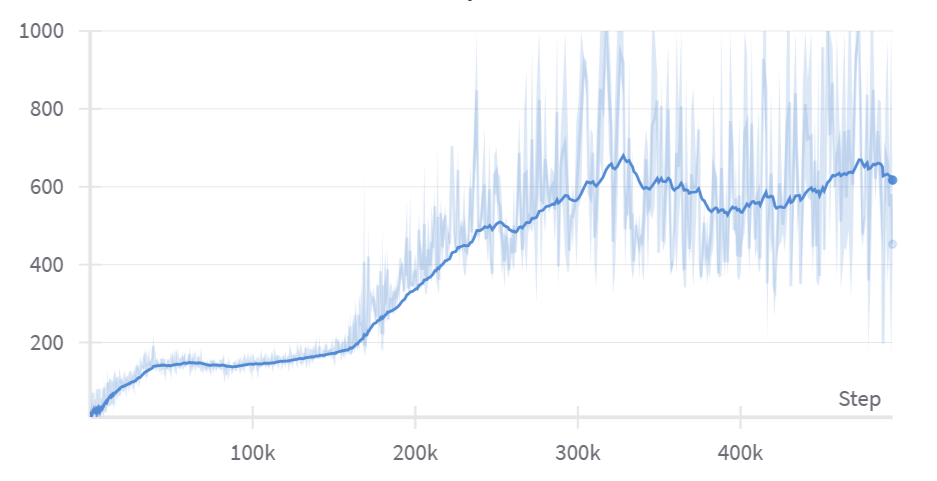
You should expect the reward to increase pretty fast initially and then plateau once the agent learns the solution "kick off for a very large initial jump, and don't think about landing". Eventually the agent gets past this plateau, and learns to land successfully without immediately falling over. Once it's at the point where it can string two jumps together, your reward should start increasing much faster.
Here is a video produced from a successful run, using the parameters above:
and here's the corresponding plot of episode lengths:
Although we've used Hopper-v4 in these examples, you might also want to try InvertedPendulum-v4 (docs here). It's a much easier environment to solve, and it's a good way to check that your implementation is working (after all if it worked for CartPole then it should work here - in fact your inverted pendulum agent should converge to a perfect solution almost instantly, no reward shaping required). You can check out the other MuJoCo environments here.
Designing your own reward from scratch
So far every environment came with its reward already defined. But the reward function is part of the problem specification: a poor choice often means the agent gets no feedback at all to learn from. A good property of a reward function is that it should be able to distinguish between different rollouts from a randomly initialized policy: At the start of training, the policy network will likely be taking completely random actions, so we require that at least some of these random rollouts receive more reward than others, so theat the training algorithm has something to latch onto at the start. For a complicated game where the agent has to, say, navigate a long and complex environment before it finds anything that doles out reward, it is unlikely the agent will learnt to do anything at all.
We've wired two more GPU environments into ENV_DICT, both runnable through the same PPOTrainer /
PPOTrainerCts you already have:
mode="mountain-car"; a discrete-actionMountainCar(uses the classic-control actor/critic).mode="pendulum"; a continuous-actionPendulum(uses the MuJoCo Gaussian actor/critic).
Worked example: reward shaping on MountainCar
In MountainCar
an underpowered car has to climb the right-hand hill, but its engine is too weak to
drive straight up; it must rock back and forth to build momentum. The native reward is
-1 on every step until it reaches the flag. That reward is sparse: almost every trajectory just
collects a flat -200, so there's no gradient telling the policy which way is better, and vanilla PPO
essentially never solves it.
The fix is reward shaping: add a term that points the agent in a helpful direction without
changing what "success" means. A principled choice is to reward the car's total mechanical energy
(kinetic + gravitational potential). For the passive dynamics this energy is conserved, so the only
way to increase it is to actively pump energy in (push in the direction you're already moving), which
is exactly the rocking behaviour needed to escape the valley. Concretely, for the dynamics
v' = v - gravity*cos(3x) the conserved energy is
(the potential term is chosen so that $-\,dE/dx$ reproduces the -gravity*cos(3x) gravity term in the
dynamics). Because GPUEnv keeps reward_function as a separate, overridable method, the shaped
reward is a couple of lines (the physics in step is untouched):
if SLOW:
    # Shape MountainCar's sparse -1 reward by rewarding total mechanical energy (kinetic + potential).
    # The agent can only raise this by pumping energy into the system, which is how it escapes the
    # valley. The dynamics are unchanged; we just scale to O(1) for a well-conditioned value function.
    def mountaincar_energy_reward(self, action):
        x, v = self.state[:, 0], self.state[:, 1]
        kinetic = 0.5 * v ** 2
        potential = (self.gravity / 3.0) * t.sin(3 * x)  # gravitational PE consistent with the dynamics
        return 1000.0 * (kinetic + potential)

    MountainCar.reward_function = mountaincar_energy_reward

    args = PPOArgs(
        env_id="MountainCar-v0",
        wandb_project_name="PPOMountainCar",
        mode="mountain-car",
        total_timesteps=30_000_000,
        num_envs=2048,
        num_steps_per_rollout=64,
        num_minibatches=4,
        lr=3e-3,
        gamma=0.99,
        ent_coef=0.01,
        vf_coef=0.5,
    )
    trainer = PPOTrainer(args)
    trainer.train()
    display(record_grid_video(trainer, kind="mountain-car"))
Exercise - design a reward function for Pendulum
The Pendulum environment is a single rigid pole attached to a pivot, actuated by
a motor at the pivot. The pole starts hanging down (with a little random perturbation) and the agent
action is the continuous space of [-2,2], applying a torque to the pivot.
The goal is to swing the pole upright and balance it pointing straight up,
then hold it there. The torque alone is insufficent to raise the pole directly under
gravity (it is too heavy), so the optimal policy will need to swing the pole back and forth.
Unlike the previous environments, Pendulum ships with no reward function
(reward_function raises NotImplementedError). You have to design one.
Here is everything you need to know about the environment (taken from the gymnasium Pendulum docs and the source.
⚠️ The above links describe the original reward function used and will spoil this exercise!
Internal state self.state is a (num_envs, 2) tensor [theta, theta_dot]:
| Index | Symbol | Meaning | Range |
|---|---|---|---|
| 0 | theta |
angle of the pole, measured from straight up (theta = 0 is balanced upright; theta = ±π is hanging straight down). Wraps around. |
[-π, π] (after wrapping) |
| 1 | theta_dot |
angular velocity | [-8, 8] |
Observation (what the policy network sees) ; a (num_envs, 3) tensor; the angle is given as
a (cos, sin) pair so the policy sees a continuous representation with no wrap discontinuity, and that
the precomputed features of $\cos(\theta)$ and $\sin(\theta)$ make it easier to learn from.
| Index | Observation | Min | Max |
|---|---|---|---|
| 0 | x = cos(theta) |
-1.0 | 1.0 |
| 1 | y = sin(theta) |
-1.0 | 1.0 |
| 2 | angular velocity | -8.0 | 8.0 |
Action; a single continuous torque applied at the pivot, in [-2.0, 2.0].
Dynamics (already implemented for you, simulating the physics of the pendulum with gravity = 10, mass = 1, length = 1, dt = 0.05). The dynamics numerically integrate the ODE that describes the pendulum's motion using Euler's method (see gpu_env.py for the implementation).
Episode; a continuing task that truncates after 200 steps (then auto-resets). Each episode starts with $\theta \sim \mathcal{U}[-\pi, \pi]$ and $\dot{\theta} \sim \mathcal{U}[-1, 1]$.
Before writing any code, play the environment yourself to build intuition for what a good policy (and therefore a good reward) looks like: open the interactive demo and try to swing the pole up and balance it using the torque controls.
Notice the demo shows you the observation (the three sliders) but deliberately shows no score; quantifying "upright and still" into a single number is exactly the design problem you're solving.
Now implement pendulum_reward below. It receives the angle, angular velocity, and applied torque
(all (num_envs,) tensors) and must return a (num_envs,) reward tensor. Consider the following:
- When should the reward be highest? (The pole upright and not spinning.)
thetawraps at±π; the helperangle_normalize(x)maps any angle into[-π, π], soangle_normalize(theta)is the signed distance from upright.- Should you discourage anything else, like spending lots of torque or spinning fast?
- The reward must be dense (informative at every state), or you'll have MountainCar's problem.
def pendulum_reward(theta: Tensor, theta_dot: Tensor, torque: Tensor) -> Tensor:
    """
    Reward for the Pendulum swing-up task. All arguments are (num_envs,) tensors:
        theta     : pole angle in radians; theta=0 is straight up, theta=±π is hanging down (wraps).
        theta_dot : angular velocity, in [-8, 8].
        torque    : the applied action, in [-2, 2].
    Returns a (num_envs,) reward tensor, larger when the pole is upright and still.
    """
    raise NotImplementedError()
# Bind your reward to the Pendulum env so `mode="pendulum"` uses it (the dynamics are untouched):
def _pendulum_reward_method(self, action):
    u = action.reshape(self.num_envs).clamp(-self.max_torque, self.max_torque)
    return pendulum_reward(self.state[:, 0], self.state[:, 1], u)

class MyPendulum(Pendulum):
    def reward_function(self, action):
        return _pendulum_reward_method(self, action)

# Register the reward-equipped subclass so `PPOTrainer`/`PPOTrainerCts` build it for mode="pendulum"
# (the base `Pendulum` deliberately raises until you supply a reward).
ENV_DICT["pendulum"] = MyPendulum
Solution
def pendulum_reward(theta: Tensor, theta_dot: Tensor, torque: Tensor) -> Tensor:
    """
    Reward for the Pendulum swing-up task. All arguments are (num_envs,) tensors:
        theta     : pole angle in radians; theta=0 is straight up, theta=±π is hanging down (wraps).
        theta_dot : angular velocity, in [-8, 8].
        torque    : the applied action, in [-2, 2].
    Returns a (num_envs,) reward tensor, larger when the pole is upright and still.
    """
    # One good choice (the canonical gym reward): a negative quadratic cost that is zero only when the
    # pole is exactly upright, motionless, and no torque is applied. angle_normalize(theta) is the
    # signed angular distance from upright, so its square penalises being away from the top; the other
    # two terms gently discourage spinning and wasting control effort.
    return -(angle_normalize(theta) ** 2 + 0.1 * theta_dot ** 2 + 0.001 * torque ** 2)
Now train it. Pendulum is small, so with thousands of parallel envs on the GPU a good reward function should cause the agent to swing the pole up and balance it in well under a minute with the provided hyperparameters. The ones provided, with the canonical reward function fromm gym, learns in <15 seconds. If your agent hasn't learned by a minute, your reward function needs some work.
if SLOW:
    args = PPOArgs(
        env_id="Pendulum-v1",
        wandb_project_name="PPOPendulum",
        mode="pendulum",
        total_timesteps=20_000_000,
        num_envs=4096,
        num_steps_per_rollout=64,
        num_minibatches=4,
        lr=3e-3,
        gamma=0.95,
        ent_coef=0.0,
        vf_coef=0.5,
    )
    trainer = PPOTrainerCts(args)
    trainer.train()
    display(record_grid_video(trainer, kind="pendulum"))
Swing-up: cart + double pendulum
For a harder continuous-control task we provide a custom cart + double-pendulum environment,
CartDoublePendulum (in gpu_env.py), and register it under mode="swing-up". A cart slides on a
finite rail and carries a double pendulum (two un-actuated poles in series). Both poles start
hanging straight down, and the agent — which can only push the cart left/right — has to swing
them up and balance them inverted, then hold that unstable equilibrium without running off the
rail. It's the classic acrobot/swing-up challenge with an extra link, so it needs a genuine
closed-loop feedback policy rather than a memorised torque sequence.
Like our other accelerated environments it inherits from GPUEnv and runs entirely on the GPU:
the equations of motion (a batched 3×3 manipulator-form linear solve) are integrated with RK4 for
thousands of carts in parallel, so a step never leaves the device. The 8-D observation is
[x, x', cos θ₁, sin θ₁, cos θ₂, sin θ₂, θ₁', θ₂'] (angles as cos/sin pairs to avoid the 2π wrap
discontinuity) and the single continuous action is the cart
force, so we reuse the same Gaussian Actor/Critic as MuJoCo (get_actor_and_critic routes
"swing-up" to get_actor_and_critic_mujoco) and train it with PPOTrainerCts.
A couple of design points worth noting:
- Randomised start. Each episode perturbs the two joint angles by a small zero-mean Gaussian
(
init_angle_noise=0.05rad) around "hanging down". The double pendulum is chaotic, so even this tiny perturbation makes every episode's trajectory diverge — the agent is forced to learn a feedback controller instead of replaying one open-loop action sequence. - Reward shaping via
reward_function.GPUEnvkeepsterminatedandreward_functionas separate, overridable methods (the physics instepis untouched), so reward shaping is a one-method subclass. The default dense reward rewards getting both poles upright (and the outer tip high), with a mild pull to the rail centre and small penalties on control effort, joint velocities, and a crash off the rail.
It trains to a clear swing-up in a couple of minutes on a single GPU:
if SLOW:
    args = PPOArgs(
        env_id="CartDoublePendulum",
        wandb_project_name="PPOSwingUp",
        mode="swing-up",
        total_timesteps=60_000_000,
        num_envs=4096,
        num_steps_per_rollout=64,
        num_minibatches=8,
        batches_per_learning_phase=4,
        lr=5e-4,
        gamma=0.99,
        gae_lambda=0.95,
        clip_coef=0.2,
        ent_coef=0.003,
        vf_coef=0.5,
    )
    trainer = PPOTrainerCts(args)
    trainer.train()
    # 4x4 grid of independent carts, each rendered from its own observation.
    display(record_grid_video(trainer, kind="swingup"))