1️⃣ Setting up our agent

Learning Objectives

• Understand the difference between the actor & critic networks, and what their roles are
• Learn about & implement generalised advantage estimation
• Build a replay memory to store & sample experiences
• Design an agent class to step through the environment & record experiences

In this section, we'll do the following:

• Define a dataclass to hold our PPO arguments
• Write functions to create our actor and critic networks (which will eventually be stored in our PPOAgent instance)
• Write a function to do generalized advantage estimation (this will be necessary when computing our objective function during the learning phase)
• Fill in our ReplayMemory class (for storing and sampling experiences)
• Fill in our PPOAgent class (a wrapper around our networks and our replay memory, which will turn them into an agent)

As a reminder, we'll be continually referring back to The 37 Implementation Details of Proximal Policy Optimization as we go through these exercises. Most of our sections wil refer to one or more of these details.

PPO Arguments

Just like for DQN, we've provided you with a dataclass containing arguments for your train_ppo function. We've also given you a function from utils to display all these arguments (including which ones you've changed). Lots of these are the same as for the DQN dataclass.

Don't worry if these don't all make sense right now, they will by the end.

@dataclass
class PPOArgs:
    # Basic / global
    seed: int = 1
    env_id: str = "CartPole-v1"
    mode: EnvType = "classic-control"

    # Wandb / logging
    use_wandb: bool = False
    video_log_freq: int | None = None
    wandb_project_name: str = "PPOCartPole"
    wandb_entity: str = None

    # Duration of different phases. With the GPU-batched CartPole we run many more parallel envs,
    # so num_envs is large; total_timesteps is sized to ~150 learning phases (~17s on a GPU,
    # CartPole is solved well before the end).
    total_timesteps: int = 10_000_000
    num_envs: int = 1024
    num_steps_per_rollout: int = 64
    num_minibatches: int = 4
    batches_per_learning_phase: int = 4

    # Optimization hyperparameters (higher LR converges in seconds with this many parallel envs)
    lr: float = 5e-3
    max_grad_norm: float = 0.5

    # RL hyperparameters
    gamma: float = 0.99

    # PPO-specific hyperparameters
    gae_lambda: float = 0.95
    clip_coef: float = 0.2
    ent_coef: float = 0.01
    vf_coef: float = 1.0

    def __post_init__(self):
        self.batch_size = self.num_steps_per_rollout * self.num_envs

        assert self.batch_size % self.num_minibatches == 0, "batch_size must be divisible by num_minibatches"
        self.minibatch_size = self.batch_size // self.num_minibatches
        self.total_phases = self.total_timesteps // self.batch_size
        self.total_training_steps = self.total_phases * self.batches_per_learning_phase * self.num_minibatches

        self.video_save_path = section_dir / "videos"


args = PPOArgs(num_minibatches=2)  # changing this also changes minibatch_size and total_training_steps
arg_help(args)

A note on the num_envs argument - note that unlike yesterday, envs will actually have multiple instances of the environment inside (we did still have this argument yesterday but it was always set to 1). From the 37 implementation details of PPO post:

In this architecture, PPO first initializes a vectorized environment envs that runs $N$ (usually independent) environments either sequentially or in parallel by leveraging multi-processes. envs presents a synchronous interface that always outputs a batch of $N$ observations from $N$ environments, and it takes a batch of $N$ actions to step the $N$ environments. When calling next_obs = envs.reset(), next_obs gets a batch of $N$ initial observations (pronounced "next observation"). PPO also initializes an environment done flag variable next_done (pronounced "next done") to an $N$-length array of zeros, where its i-th element next_done[i] has values of 0 or 1 which corresponds to the $i$-th sub-environment being not done and done, respectively.

Actor-Critic Implementation (detail #2)

PPO requires two networks, an actor and a critic. The actor is the most important one; its job is to learn an optimal policy $\pi_\theta(a_t \mid s_t)$ (it does this by training on the clipped surrogate objective function, which is essentially a direct estimation of the discounted sum of future rewards with some extra bells and whistles thrown in). Estimating this also requires estimating the advantage function $A_\theta(s_t, a_t)$, which in requires estimating the values $V_\theta(s_t)$ - this is why we need a critic network, which learns $V_\theta(s_t)$ by minimizing the TD residual (in a similar way to how our Q-network learned the $Q(s_t, a_t)$ values).

Exercise - implement get_actor_and_critic

You should implement the Agent class according to the diagram. We are doing separate Actor and Critic networks because detail #13 notes that is performs better than a single shared network in simple environments. Use layer_init to initialize each Linear, overriding the standard deviation argument std according to the diagram (when not specified, you should be using the default value of std=np.sqrt(2)).

We've given you a "high level function" get_actor_and_critic which calls one of three possible functions, depending on the mode argument. You'll implement the other two modes later. This is one way to keep our code modular.

def layer_init(layer: nn.Linear, std=np.sqrt(2), bias_const=0.0):
    t.nn.init.orthogonal_(layer.weight, std)
    t.nn.init.constant_(layer.bias, bias_const)
    return layer


def get_actor_and_critic(
    envs: gym.vector.SyncVectorEnv,
    mode: EnvType = "classic-control",
) -> tuple[nn.Module, nn.Module]:
    """
    Returns (actor, critic), the networks used for PPO, in one of 3 different modes.
    """
    assert mode in ENV_DICT

    obs_shape = envs.single_observation_space.shape
    num_obs = np.array(obs_shape).prod()
    num_actions = (
        envs.single_action_space.n
        if isinstance(envs.single_action_space, gym.spaces.Discrete)
        else np.array(envs.single_action_space.shape).prod()
    )

    if mode in ("classic-control", "mountain-car", "probe"):
        # mountain-car (Discrete(3)) and the probe envs are also discrete classic-control tasks, so
        # they reuse this network.
        actor, critic = get_actor_and_critic_classic(num_obs, num_actions)
    if mode == "atari":
        actor, critic = get_actor_and_critic_atari(obs_shape, num_actions)  # you'll implement these later
    if mode in ("mujoco", "swing-up", "pendulum"):
        # swing-up (cart + double-pendulum) and pendulum are continuous-action tasks, so they reuse
        # the MuJoCo Gaussian actor/critic.
        actor, critic = get_actor_and_critic_mujoco(num_obs, num_actions)  # you'll implement these later

    return actor.to(device), critic.to(device)


def get_actor_and_critic_classic(num_obs: int, num_actions: int):
    """
    Returns (actor, critic) in the "classic-control" case, according to diagram above.
    """
    raise NotImplementedError()


tests.test_get_actor_and_critic(get_actor_and_critic, mode="classic-control")

def layer_init(layer: nn.Linear, std=np.sqrt(2), bias_const=0.0):
    t.nn.init.orthogonal_(layer.weight, std)
    t.nn.init.constant_(layer.bias, bias_const)
    return layer


def get_actor_and_critic(
    envs: gym.vector.SyncVectorEnv,
    mode: EnvType = "classic-control",
) -> tuple[nn.Module, nn.Module]:
    """
    Returns (actor, critic), the networks used for PPO, in one of 3 different modes.
    """
    assert mode in ENV_DICT

    obs_shape = envs.single_observation_space.shape
    num_obs = np.array(obs_shape).prod()
    num_actions = (
        envs.single_action_space.n
        if isinstance(envs.single_action_space, gym.spaces.Discrete)
        else np.array(envs.single_action_space.shape).prod()
    )

    if mode in ("classic-control", "mountain-car", "probe"):
        # mountain-car (Discrete(3)) and the probe envs are also discrete classic-control tasks, so
        # they reuse this network.
        actor, critic = get_actor_and_critic_classic(num_obs, num_actions)
    if mode == "atari":
        actor, critic = get_actor_and_critic_atari(obs_shape, num_actions)  # you'll implement these later
    if mode in ("mujoco", "swing-up", "pendulum"):
        # swing-up (cart + double-pendulum) and pendulum are continuous-action tasks, so they reuse
        # the MuJoCo Gaussian actor/critic.
        actor, critic = get_actor_and_critic_mujoco(num_obs, num_actions)  # you'll implement these later

    return actor.to(device), critic.to(device)


def get_actor_and_critic_classic(num_obs: int, num_actions: int):
    """
    Returns (actor, critic) in the "classic-control" case, according to diagram above.
    """
    actor = nn.Sequential(
        layer_init(nn.Linear(num_obs, 64)),
        nn.Tanh(),
        layer_init(nn.Linear(64, 64)),
        nn.Tanh(),
        layer_init(nn.Linear(64, num_actions), std=0.01),
    )
    critic = nn.Sequential(
        layer_init(nn.Linear(num_obs, 64)),
        nn.Tanh(),
        layer_init(nn.Linear(64, 64)),
        nn.Tanh(),
        layer_init(nn.Linear(64, 1), std=1.0),
    )
    return actor, critic


tests.test_get_actor_and_critic(get_actor_and_critic, mode="classic-control")

Generalized Advantage Estimation (detail #5)

The advantage function $A_\theta(s_t, a_t)$ is defined as $Q_\theta(s_t, a_t) - V_\theta(s_t)$, i.e. it's the difference between expected future reward when we take action $a_t$ vs taking the expected action according to policy $\pi_\theta$ from that point onwards. It's an important part of our objective function, because it tells us whether we should try and take more or less of action $a_t$ in state $s_t$. A positive (negative) advantage indicates that this is a better (worse) action than $\pi$ would have done

Our critic estimates $V_\theta(s_t)$, but we need $A_\theta(s_t, a_t)$, so we have to estimate it from the rewards and values we actually observe. The question is how far into the future to look, and the answer is a bias-variance tradeoff.

The 1-step estimate

The most local estimate uses a single observed reward and then falls back on the critic for everything after that:

This quantity $\delta_t$ - the TD residual - is itself an advantage estimate. If the critic were exact then $\mathbb{E}[r_t + \gamma V_\theta(s_{t+1})] = Q_\theta(s_t, a_t)$, so $\mathbb{E}[\delta_t] = A_\theta(s_t, a_t)$. It has low variance (it only contains one random reward) but is biased, because it leans entirely on the critic's imperfect estimate of everything beyond a single step.

The n-step estimate

We can trust the critic less by rolling out $n$ real rewards before bootstrapping with $V_\theta$:

As $n$ grows we use more real reward and rely less on the critic, so bias falls but variance rises (we're now summing many random rewards). In the limit $n \to \infty$ we get the Monte-Carlo advantage - the full realized return minus $V_\theta(s_t)$ - which is unbiased but high-variance. Usefully, each n-step estimate is just a discounted sum of TD residuals (the $V$ terms telescope):

GAE: averaging over all $n$

Rather than commit to a single $n$, generalized advantage estimation (GAE) takes an exponentially-weighted average of every n-step estimate, with weight $\propto \lambda^{n-1}$ for a decay parameter $\lambda \in [0, 1]$. This average collapses to a clean geometric sum of TD residuals:

Now $\lambda$ slides smoothly along the bias-variance tradeoff: $\lambda = 0$ recovers the 1-step estimate $\hat{A}_t = \delta_t$ (low variance, high bias), and $\lambda = 1$ recovers the Monte-Carlo estimate (high variance, low bias). In practice we use something like $\lambda = 0.95$, keeping most of the variance reduction of the critic while still folding in many real rewards.

GAE also helps the critic: instead of regressing $V_\theta(s_t)$ onto a 1-step target (as we effectively did in SARSA), we'll regress it onto $\hat{A}^{\text{GAE}(\lambda)}_t + V_\theta(s_t)$, a lookahead target that incorporates many future steps. This improves stability and speeds up convergence.

Computing it in practice

Two practical points. First, a rollout has finite length $T$, so the sum is truncated at $\delta_{T-1}$. Second, we must not bootstrap across episode boundaries: if the episode terminates at the next step ($d_{t+1} = 1$) there is no $V_\theta(s_{t+1})$ to look ahead to, so the residual is just $\delta_t = r_t - V_\theta(s_t)$ and we cut off the future advantage. Both points are handled by computing GAE in a single reverse pass with the recursion:

Exercise - implement compute_advantages

Below, you should fill in compute_advantages. We recommend using a reversed for loop over $t$ to get it working, and using the recursive formula for GAE given above - don't worry about trying to vectorize it.

Tip - make sure you understand what the indices are of the tensors you've been given! The tensors rewards, values and terminated contain $r_t$, $V(s_t)$ and $d_t$ respectively for all $t = 0, 1, ..., T-1$, and next_value, next_terminated are the values $V(s_T)$ and $d_T$ respectively (required for the calculation of the very last advantage $A_{T-1}$).

@t.inference_mode()
def compute_advantages(
    next_value: Float[Tensor, "num_envs"],
    next_terminated: Bool[Tensor, "num_envs"],
    rewards: Float[Tensor, "buffer_size num_envs"],
    values: Float[Tensor, "buffer_size num_envs"],
    terminated: Bool[Tensor, "buffer_size num_envs"],
    gamma: float,
    gae_lambda: float,
) -> Float[Tensor, "buffer_size num_envs"]:
    """
    Compute advantages using Generalized Advantage Estimation.
    """
    raise NotImplementedError()


tests.test_compute_advantages(compute_advantages)

@t.inference_mode()
def compute_advantages(
    next_value: Float[Tensor, "num_envs"],
    next_terminated: Bool[Tensor, "num_envs"],
    rewards: Float[Tensor, "buffer_size num_envs"],
    values: Float[Tensor, "buffer_size num_envs"],
    terminated: Bool[Tensor, "buffer_size num_envs"],
    gamma: float,
    gae_lambda: float,
) -> Float[Tensor, "buffer_size num_envs"]:
    """
    Compute advantages using Generalized Advantage Estimation.
    """
    T = values.shape[0]
    terminated = terminated.float()
    next_terminated = next_terminated.float()

    # Get tensors of V(s_{t+1}) and d_{t+1} for all t = 0, 1, ..., T-1
    next_values = t.concat([values[1:], next_value[None, :]])
    next_terminated = t.concat([terminated[1:], next_terminated[None, :]])

    # Compute deltas: \delta_t = r_t + (1 - d_{t+1}) \gamma V(s_{t+1}) - V(s_t)
    deltas = rewards + gamma * next_values * (1.0 - next_terminated) - values

    # Compute advantages using the recursive formula, starting with advantages[T-1] = deltas[T-1]
    # and working backwards.
    advantages = t.zeros_like(deltas)
    advantages[-1] = deltas[-1]
    for s in reversed(range(T - 1)):
        advantages[s] = deltas[s] + gamma * gae_lambda * (1.0 - terminated[s + 1]) * advantages[s + 1]

    return advantages

Replay Memory

Our replay memory has some similarities to the replay buffer from yesterday, as well as some important differences.

Sampling method

Yesterday, we continually updated our buffer and sliced off old data, and each time we called sample we'd take a randomly ordered subset of that data (with replacement).

With PPO, we alternate between rollout and learning phases. In rollout, we fill our replay memory entirely. In learning, we call get_minibatches to return the entire contents of the replay memory, but randomly shuffled and sorted into minibatches. In this way, we update on every experience, not just random samples. In fact, we'll update on each experience more than once, since we'll repeat the process of (generate minibatches, update on all of them) batches_per_learning_phase times during each learning phase.

New variables

We store some of the same variables as before - $(s_t, a_t, d_t)$, but with the addition of 3 new variables: the logprobs $\pi(a_t\mid s_t)$, the advantages $A_t$ and the returns. Explaining these two variables and why we need them:

• logprobs are calculated from the logit outputs of our actor.agent network, corresponding to the actions $a_t$ which our agent actually chose.
  • These are necessary for calculating the clipped surrogate objective (see equation $(7)$ on page page 3 in the PPO Algorithms paper), which as we'll see later makes sure the agent isn't rewarded for changing its policy an excessive amount.
• advantages are the terms $\hat{A}_t$, computed using our function compute_advantages from earlier.
  • Again, these are used in the calculation of the clipped surrogate objective.
• returns are given by the formula returns = advantages + values - see detail #9.
  • They are used to train the value network, in a way which is equivalent to minimizing the TD residual loss used in DQN.

Don't worry if you don't understand all of this now, we'll get to all these variables later.

Exercise - implement minibatch_indices

We'll start by implementing the get_minibatch_indices function, as described in detail #6. This will give us a list of length num_minibatches = batch_size // minibatch_size indices, each of length minibatch_size, and which collectively represent a permutation of the indices [0, 1, ..., batch_size - 1] where batch_size = num_minibatches * minibatch_size. To help visualize how this works to create our minibatches, we've included a diagram:

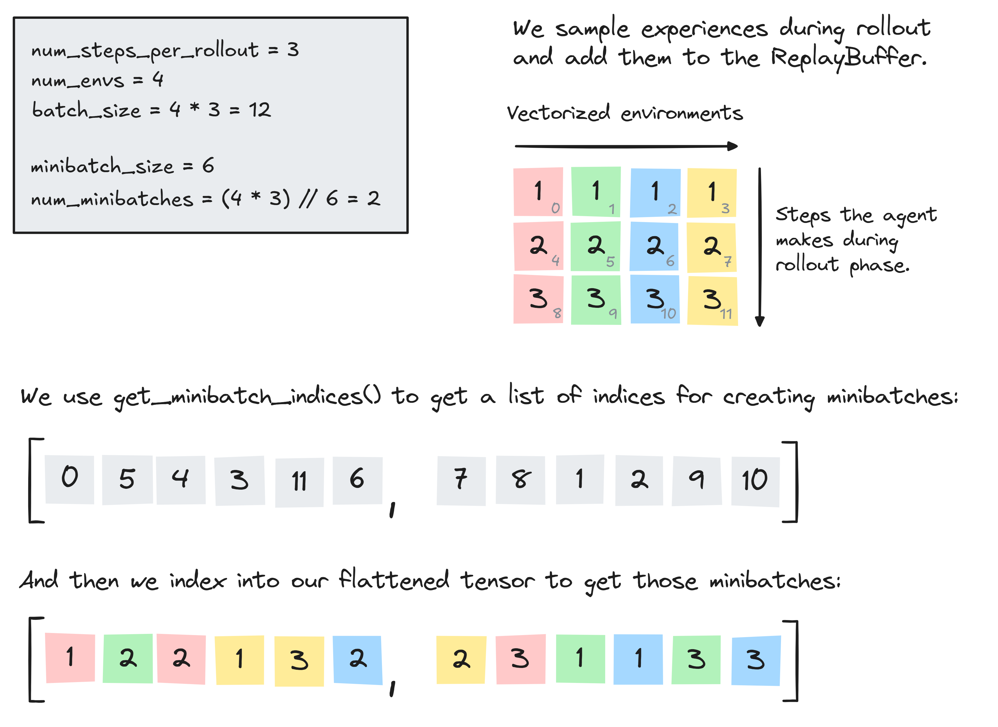
The test code below should also make it clear what your function should be returning.

def get_minibatch_indices(rng: Generator, batch_size: int, minibatch_size: int) -> list[np.ndarray]:
    """
    Return a list of length `num_minibatches`, where each element is an array of `minibatch_size` and the union of all
    the arrays is the set of indices [0, 1, ..., batch_size - 1] where `batch_size = num_steps_per_rollout * num_envs`.
    """
    assert batch_size % minibatch_size == 0
    raise NotImplementedError()


rng = np.random.default_rng(0)

batch_size = 12
minibatch_size = 6
# num_minibatches = batch_size // minibatch_size = 2

indices = get_minibatch_indices(rng, batch_size, minibatch_size)

assert isinstance(indices, list)
assert all(isinstance(x, np.ndarray) for x in indices)
assert np.array(indices).shape == (2, 6)
assert sorted(np.unique(indices)) == [0, 1, 2, 3, 4, 5, 6, 7, 8, 9, 10, 11]
print("All tests in `test_minibatch_indexes` passed!")

def get_minibatch_indices(rng: Generator, batch_size: int, minibatch_size: int) -> list[np.ndarray]:
    """
    Return a list of length `num_minibatches`, where each element is an array of `minibatch_size` and the union of all
    the arrays is the set of indices [0, 1, ..., batch_size - 1] where `batch_size = num_steps_per_rollout * num_envs`.
    """
    assert batch_size % minibatch_size == 0
    num_minibatches = batch_size // minibatch_size
    indices = rng.permutation(batch_size).reshape(num_minibatches, minibatch_size)
    return list(indices)

ReplayMemory class

Next, we've given you the ReplayMemory class. This follows a very similar structure to the DQN equivalent ReplayBuffer yesterday, with a bit of added complexity. We'll highlight the key differences below:

• There's no [-self.buffer_size:] slicing like there was in the DQN buffer yesterday. That's because rather than continually adding to our buffer and removing the oldest data, we'll iterate through a process of (fill entire memory, generate a bunch of minibatches from that memory and train on them, empty the memory, repeat).
• The get_minibatches method computes the advantages and returns. This isn't really in line with the SoC (separation of concerns) principle, but this is the easiest place to compute them because we can't do it after we sample the minibatches.
• A single learning phase involves creating num_minibatches = batch_size // minibatch_size minibatches and training on each of them, and then repeating this process batches_per_learning_phase times. So the total number of minibaches per learning phase is batches_per_learning_phase * num_minibatches.

@dataclass
class ReplayMinibatch:
    """
    Samples from the replay memory, converted to PyTorch for use in neural network training.

    Data is equivalent to (s_t, a_t, logpi(a_t|s_t), A_t, A_t + V(s_t), d_{t+1})
    """

    obs: Float[Tensor, " minibatch_size *obs_shape"]
    actions: Int[Tensor, " minibatch_size *action_shape"]
    logprobs: Float[Tensor, " minibatch_size"]
    advantages: Float[Tensor, " minibatch_size"]
    returns: Float[Tensor, " minibatch_size"]
    terminated: Bool[Tensor, " minibatch_size"]


class ReplayMemory:
    """
    Contains buffer; has a method to sample from it to return a ReplayMinibatch object.
    """

    rng: Generator
    obs: Float[Arr, " buffer_size num_envs *obs_shape"]
    actions: Int[Arr, " buffer_size num_envs *action_shape"]
    logprobs: Float[Arr, " buffer_size num_envs"]
    values: Float[Arr, " buffer_size num_envs"]
    rewards: Float[Arr, " buffer_size num_envs"]
    terminated: Bool[Arr, " buffer_size num_envs"]

    def __init__(
        self,
        num_envs: int,
        obs_shape: tuple,
        action_shape: tuple,
        batch_size: int,
        minibatch_size: int,
        batches_per_learning_phase: int,
        seed: int = 42,
    ):
        self.num_envs = num_envs
        self.obs_shape = obs_shape
        self.action_shape = action_shape
        self.batch_size = batch_size
        self.minibatch_size = minibatch_size
        self.batches_per_learning_phase = batches_per_learning_phase
        self.rng = np.random.default_rng(seed)
        self.reset()

    def reset(self):
        """Resets all stored experiences, ready for new ones to be added to memory. We keep one
        list of per-step GPU tensors per field and stack them once at sampling time, so nothing
        leaves the GPU during a rollout."""
        self.obs = []
        self.actions = []
        self.logprobs = []
        self.values = []
        self.rewards = []
        self.terminated = []

    def add(
        self,
        obs: Float[Arr, " num_envs *obs_shape"],
        actions: Int[Arr, " num_envs *action_shape"],
        logprobs: Float[Arr, " num_envs"],
        values: Float[Arr, " num_envs"],
        rewards: Float[Arr, " num_envs"],
        terminated: Bool[Arr, " num_envs"],
    ) -> None:
        """Add a batch of transitions to the replay memory. All inputs are GPU tensors and stay on
        the GPU (we just append the references; they're stacked at sampling time)."""
        # Check shapes & datatypes
        for data, expected_shape in zip(
            [obs, actions, logprobs, values, rewards, terminated],
            [self.obs_shape, self.action_shape, (), (), (), ()],
        ):
            assert isinstance(data, Tensor)
            assert data.shape == (self.num_envs, *expected_shape)

        # Append this step's tensors (no concatenation / host transfer)
        self.obs.append(obs)
        self.actions.append(actions)
        self.logprobs.append(logprobs)
        self.values.append(values)
        self.rewards.append(rewards)
        self.terminated.append(terminated)

    def get_minibatches(
        self, next_value: Tensor, next_terminated: Tensor, gamma: float, gae_lambda: float
    ) -> list[ReplayMinibatch]:
        """
        Returns a list of minibatches. Each minibatch has size `minibatch_size`, and the union over
        all minibatches is `batches_per_learning_phase` copies of the entire replay memory.
        """
        # Stack the per-step tensors into shape (buffer_size, num_envs, ...)
        obs, actions, logprobs, values, rewards, terminated = (
            t.stack(x)
            for x in [
                self.obs,
                self.actions,
                self.logprobs,
                self.values,
                self.rewards,
                self.terminated,
            ]
        )

        # Compute advantages & returns
        advantages = compute_advantages(next_value, next_terminated, rewards, values, terminated, gamma, gae_lambda)
        returns = advantages + values

        # Return a list of minibatches (indices are moved onto the GPU to index the on-device data)
        minibatches = []
        for _ in range(self.batches_per_learning_phase):
            for indices in get_minibatch_indices(self.rng, self.batch_size, self.minibatch_size):
                idx = t.as_tensor(indices, dtype=t.long, device=device)
                minibatches.append(
                    ReplayMinibatch(
                        *[
                            data.flatten(0, 1)[idx]
                            for data in [obs, actions, logprobs, advantages, returns, terminated]
                        ]
                    )
                )

        # Reset memory (since we only need to call this method once per learning phase)
        self.reset()

        return minibatches

Like before, here's some code to generate and plot observations.

The first plot shows the current observations $s_t$ (with dotted lines indicating a terminated episode $d_{t+1} = 1$). The solid lines indicate the transition between different environments in envs (because unlike yesterday, we're actually using more than one environment in our SyncVectorEnv). There are batch_size = num_steps_per_rollout * num_envs = 128 * 2 = 256 observations in total, with 128 coming from each environment.

The second plot shows a single minibatch of sampled experiences from full memory. Each minibatch has size minibatch_size = 128, and minibatches contains in total batches_per_learning_phase * (batch_size // minibatch_size) = 2 * 2 = 4 minibatches.

Note that we don't need to worry about terminal observations here, because we're not actually logging next_obs (unlike DQN, this won't be part of our loss function).

num_steps_per_rollout = 128
num_envs = 2
batch_size = num_steps_per_rollout * num_envs  # 256

minibatch_size = 128
num_minibatches = batch_size // minibatch_size  # 2

batches_per_learning_phase = 2

envs = CartPole(num_envs=num_envs)  # GPU-batched env: reset()/step() return on-device tensors
memory = ReplayMemory(num_envs, (4,), (), batch_size, minibatch_size, batches_per_learning_phase)

logprobs = values = t.zeros(num_envs, device=device)  # dummy values, just so we can see demo of plot
obs, _ = envs.reset()

for i in range(num_steps_per_rollout):  # the locally-defined 128, matching this cell's batch_size
    # Choose a random action and step the env (actions are an on-device tensor for the batched env)
    actions = t.randint(0, envs.single_action_space.n, (num_envs,), device=device)
    next_obs, rewards, terminated, truncated, infos = envs.step(actions)

    # Add experience to memory (everything is already an on-device tensor)
    memory.add(obs, actions, logprobs, values, rewards, terminated)
    obs = next_obs

plot_cartpole_obs_and_dones(
    t.stack(memory.obs).cpu(),
    t.stack(memory.terminated).cpu(),
    title="Current obs s<sub>t</sub><br>Dotted lines indicate d<sub>t+1</sub> = 1, solid lines are environment separators",
)

next_value = next_done = t.zeros(envs.num_envs).to(device)  # dummy values, just so we can see demo of plot
minibatches = memory.get_minibatches(next_value, next_done, gamma=0.99, gae_lambda=0.95)

plot_cartpole_obs_and_dones(
    minibatches[0].obs.cpu(),
    minibatches[0].terminated.cpu(),
    title="Current obs (sampled)<br>this is what gets fed into our model for training",
)

PPO Agent

As the final task in this section, you should fill in the agent's play_step method. This is conceptually similar to what you did during DQN, but with a few key differences:

• In DQN we selected actions based on our Q-network & an epsilon-greedy policy, but instead your actions will be generated directly from your actor network
• Here, you'll have to compute the extra data logprobs and values, which we didn't have to deal with in DQN

Exercise - implement PPOAgent

A few tips:

• When sampling actions (and calculating logprobs), you might find torch.distributions.categorical.Categorical useful. If logits is a 2D tensor of shape (N, k) containing a batch of logit vectors and dist = Categorical(logits=logits), then:
  • actions = dist.sample() will give you a vector of N sampled actions (which will be integers in the range [0, k)),
  • logprobs = dist.log_prob(actions) will give you a vector of the N logprobs corresponding to the sampled actions
• Make sure to use inference mode when using obs to compute logits and values, since all you're doing here is getting experiences for your memory - you aren't doing gradient descent based on these values.
• Check the shape of your arrays when adding them to memory (the add method has lots of assert statements here to help you), and also make sure that they are arrays not tensors by calling .cpu().numpy() on them.
• Remember to update self.next_obs and self.next_terminated at the end of the function!

class PPOAgent:
    critic: nn.Sequential
    actor: nn.Sequential

    def __init__(
        self,
        envs: gym.vector.SyncVectorEnv,
        actor: nn.Module,
        critic: nn.Module,
        memory: ReplayMemory,
    ):
        super().__init__()
        self.envs = envs
        self.actor = actor
        self.critic = critic
        self.memory = memory

        self.step = 0  # Tracking number of steps taken (across all environments)
        self.next_obs = t.tensor(envs.reset()[0], device=device, dtype=t.float)  # need starting obs (in tensor form)
        self.next_terminated = t.zeros(envs.num_envs, device=device, dtype=t.bool)  # need starting termination=False

    def play_step(self) -> list[dict]:
        """
        Carries out a single interaction step between the agent and the environment, and adds
        results to the replay memory.

        Returns the list of info dicts returned from `self.envs.step`.
        """
        # Get newest observations (i.e. where we're starting from)
        obs = self.next_obs
        terminated = self.next_terminated

        raise NotImplementedError()

        self.step += self.envs.num_envs
        return infos

    def get_minibatches(self, gamma: float, gae_lambda: float) -> list[ReplayMinibatch]:
        """
        Gets minibatches from the replay memory, and resets the memory
        """
        with t.inference_mode():
            next_value = self.critic(self.next_obs).flatten()
        minibatches = self.memory.get_minibatches(next_value, self.next_terminated, gamma, gae_lambda)
        self.memory.reset()
        return minibatches


tests.test_ppo_agent(PPOAgent)

class PPOAgent:
    critic: nn.Sequential
    actor: nn.Sequential

    def __init__(
        self,
        envs: gym.vector.SyncVectorEnv,
        actor: nn.Module,
        critic: nn.Module,
        memory: ReplayMemory,
    ):
        super().__init__()
        self.envs = envs
        self.actor = actor
        self.critic = critic
        self.memory = memory

        self.step = 0  # Tracking number of steps taken (across all environments)
        self.next_obs = t.tensor(envs.reset()[0], device=device, dtype=t.float)  # need starting obs (in tensor form)
        self.next_terminated = t.zeros(envs.num_envs, device=device, dtype=t.bool)  # need starting termination=False

    def play_step(self) -> list[dict]:
        """
        Carries out a single interaction step between the agent and the environment, and adds
        results to the replay memory.

        Returns the list of info dicts returned from `self.envs.step`.
        """
        # Get newest observations (i.e. where we're starting from)
        obs = self.next_obs
        terminated = self.next_terminated

        # Compute logits based on newest observation, and use it to get an action distribution we sample from.
        with t.inference_mode():
            logits = self.actor(obs)
        dist = Categorical(logits=logits)
        actions = dist.sample()


        next_obs, rewards, next_terminated, next_truncated, infos = self.envs.step(actions)

        # Calculate logprobs and values, and add this all to replay memory
        logprobs = dist.log_prob(actions)
        with t.inference_mode():
            values = self.critic(obs).flatten()
        self.memory.add(obs, actions, logprobs, values, rewards, terminated)

        self.next_obs = next_obs
        self.next_terminated = next_terminated

        self.step += self.envs.num_envs
        return infos

    def get_minibatches(self, gamma: float, gae_lambda: float) -> list[ReplayMinibatch]:
        """
        Gets minibatches from the replay memory, and resets the memory
        """
        with t.inference_mode():
            next_value = self.critic(self.next_obs).flatten()
        minibatches = self.memory.get_minibatches(next_value, self.next_terminated, gamma, gae_lambda)
        self.memory.reset()
        return minibatches