2️⃣ Exploration & Probes

Exploration

DQN makes no attempt to explore intelligently. The exploration strategy is the same as for Q-Learning: agents take a random action with probability epsilon, but now we gradually decrease epsilon. The Q-network is also randomly initialized (rather than initialized with zeros), so its predictions of what is the best action to take are also pretty random to start.

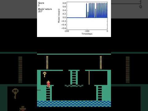
Some games like Montezuma's Revenge have sparse rewards that require more advanced exploration methods to obtain. The player is required to collect specific keys to unlock specific doors, but unlike humans, DQN has no prior knowledge about what a key or a door is, and it turns out that bumbling around randomly has too low of a probability of correctly matching a key to its door. Even if the agent does manage to do this, the long separation between finding the key and going to the door makes it hard to learn that picking the key up was important.

As a result, DQN scored an embarrassing 0% of average human performance on this game.

Reward Shaping

One solution to sparse rewards is to use human knowledge to define auxiliary reward functions that are more dense and made the problem easier (in exchange for leaking in side knowledge and making the algorithm more specific to the problem at hand). What could possibly go wrong?

The canonical example is for a game called CoastRunners, where the goal was given to maximize the score (hoping that the agent would learn to race around the map). Instead, it found it could gain more score by driving in a loop picking up power-ups just as they respawn, crashing and setting the boat alight in the process.

Reward Hacking

For Montezuma's Revenge, the reward was shaped by giving a small reward for picking up the key. One time this was tried, the reward was given slightly too early and the agent learned it could go close to the key without quite picking it up, obtain the auxiliary reward, and then back up and repeat.

A collected list of examples of Reward Hacking can be found here.

Advanced Exploration

It would be better if the agent didn't require these auxiliary rewards to be hardcoded by humans, but instead only relied on other signals from the environment that a state might be worth exploring. One idea is that a state which is "surprising" or "novel" (according to the agent's current belief of how the environment works) in some sense might be valuable. Designing an agent to be innately curious presents a potential solution to exploration, as the agent will focus exploration in areas it is unfamiliar with. In 2018, OpenAI released Random Network Distillation which made progress in formalizing this notion, by measuring the agent's ability to predict the output of a neural network on visited states. States that are hard to predict are poorly explored, and thus highly rewarded. In 2019, an excellent paper First return, then explore found an even better approach. Such reward shaping can also be gamed, leading to the noisy TV problem, where agents that seek novelty become entranced by a source of randomness in the environment (like a analog TV out of tune displaying white noise), and ignore everything else in the environment.

Exercise - implement linear scheduler

For now, implement the basic linearly decreasing exploration schedule.

def linear_schedule(
    current_step: int,
    start_e: float,
    end_e: float,
    exploration_fraction: float,
    total_timesteps: int,
) -> float:
    """
    Return the appropriate epsilon for the current step.

    Epsilon should be start_e at step 0 and decrease linearly to end_e at step (exploration_fraction
    * total_timesteps). In other words, we are in "explore mode" with start_e >= epsilon >= end_e
    for the first `exploration_fraction` fraction of total timesteps, and then stay at end_e for the
    rest of training.
    """
    raise NotImplementedError()


epsilons = [
    linear_schedule(step, start_e=1.0, end_e=0.05, exploration_fraction=0.5, total_timesteps=500)
    for step in range(500)
]
line(
    epsilons,
    labels={"x": "steps", "y": "epsilon"},
    title="Probability of random action",
    height=400,
    width=600,
)

tests.test_linear_schedule(linear_schedule)

def linear_schedule(
    current_step: int,
    start_e: float,
    end_e: float,
    exploration_fraction: float,
    total_timesteps: int,
) -> float:
    """
    Return the appropriate epsilon for the current step.

    Epsilon should be start_e at step 0 and decrease linearly to end_e at step (exploration_fraction
    * total_timesteps). In other words, we are in "explore mode" with start_e >= epsilon >= end_e
    for the first `exploration_fraction` fraction of total timesteps, and then stay at end_e for the
    rest of training.
    """
    return start_e + (end_e - start_e) * min(current_step / (exploration_fraction * total_timesteps), 1)

Epsilon Greedy Policy

In DQN, the policy is implicitly defined by the Q-network: we take the action with the maximum predicted reward. This gives a bias towards optimism. By estimating the maximum of a set of values $v_1, \ldots, v_n$ using the maximum of some noisy estimates $\hat{v}_1, \ldots, \hat{v}_n$ with $\hat{v}_i \approx v_i$, we get unlucky and get very large positive noise on some samples, which the maximum then chooses. Hence, the agent will choose actions that the Q-network is overly optimistic about.

See Sutton and Barto, Section 6.7 if you'd like a more detailed explanation, or the original Double Q-Learning paper which notes this maximisation bias, and introduces a method to correct for it using two separate Q-value estimators, each used to update the other.

Exercise - implement the epsilon greedy policy

Each environment decides independently whether to explore: environment $i$ takes a uniformly random action with probability $\varepsilon$, and the greedy action $\arg\max_a Q(o_t, a)$ otherwise. Since some environments will almost always want the greedy action, just always do the forward pass, then use t.where to pick per environment.

Other tips:

• Work with the torch random number generator rng that we've provided, rather than the global RNG. t.rand(size, generator=rng, device=device) gives uniform random numbers in $[0,1)$, and t.randint(0, n, size, generator=rng, device=device) gives random integers in the range $0, 1, \ldots, n-1$.
• Use envs.single_action_space.n to get the number of actions.

def epsilon_greedy_policy(
    envs: CartPole,
    q_network: QNetwork,
    rng: t.Generator,
    obs: Float[Tensor, " num_envs *obs_shape"],
    epsilon: float,
) -> Int[Tensor, " num_envs"]:
    """
    For each environment independently: with probability epsilon take a random action, otherwise take the greedy
    action according to the q_network.

    Inputs:
        envs:       The batched environment we're acting in
        q_network:  The QNetwork used to approximate the Q-value function
        rng:        A torch random number generator
        obs:        The current observation for each environment, shape (num_envs, *obs_shape)
        epsilon:    The probability of taking a random action

    Returns:
        actions:    The sampled action for each environment, shape (num_envs,).
    """
    raise NotImplementedError()


tests.test_epsilon_greedy_policy(epsilon_greedy_policy)

def epsilon_greedy_policy(
    envs: CartPole,
    q_network: QNetwork,
    rng: t.Generator,
    obs: Float[Tensor, " num_envs *obs_shape"],
    epsilon: float,
) -> Int[Tensor, " num_envs"]:
    """
    For each environment independently: with probability epsilon take a random action, otherwise take the greedy
    action according to the q_network.

    Inputs:
        envs:       The batched environment we're acting in
        q_network:  The QNetwork used to approximate the Q-value function
        rng:        A torch random number generator
        obs:        The current observation for each environment, shape (num_envs, *obs_shape)
        epsilon:    The probability of taking a random action

    Returns:
        actions:    The sampled action for each environment, shape (num_envs,).
    """
    num_envs = obs.shape[0]
    num_actions = envs.single_action_space.n
    with t.no_grad():
        greedy_actions = q_network(obs).argmax(dim = -1)
    is_explore = t.rand(num_envs, generator=rng, device=obs.device) < epsilon
    random_actions = t.randint(0, num_actions, (num_envs,), generator=rng, device=obs.device)
    return t.where(is_explore, random_actions, greedy_actions)

Probe Environments

Extremely simple probe environments are a great way to debug your algorithm. Ours live in chapter2_rl/exercises/gpu_probe.py, but we've copied one in for your convenience.

# Don't copy in this code, just for a demonstration
class Probe1(gym.Env):
    """
    Vectorized Probe1: One action, observation of [0.0], one timestep long, +1 reward.

    We expect the agent to rapidly learn that the value of the constant [0.0] observation is +1.0.
    Note we're using a continuous observation space for consistency with CartPole.
    """

    action_space: Discrete
    observation_space: Box

    def __init__(self, num_envs: int = 3, seed: int = 0, device: str | t.device = device):
        super().__init__()
        self.num_envs = num_envs
        self.device = t.device(device)

        self.observation_space = Box(np.array([0.0], dtype=np.float32), np.array([0.0], dtype=np.float32))
        self.action_space = Discrete(1)
        self.single_observation_space = self.observation_space  # vector-env style aliases
        self.single_action_space = self.action_space

        self.state = t.zeros([self.num_envs, 1], dtype=t.float32, device=self.device)

    def step(self, action: t.Tensor) -> tuple[t.Tensor, t.Tensor, t.Tensor, t.Tensor, dict]:
        reward = t.ones([self.num_envs], dtype=t.float32, device=self.device)
        terminated = t.ones([self.num_envs], dtype=t.bool, device=self.device)
        truncated = t.zeros([self.num_envs], dtype=t.bool, device=self.device)

        # Every env terminates each step; the auto-reset state is identical ([0.0]).
        infos = {"final_observation": self.state.clone()}
        return self.state.clone(), reward, terminated, truncated, infos

    def reset(self, *, seed: int | None = None, options=None) -> tuple[t.Tensor, dict]:
        self.state = t.zeros([self.num_envs, 1], dtype=t.float32, device=self.device)
        return self.state.clone(), {}

Let's try and break down how this environment works. We see that the function step always returns the same thing. The observation and reward are always the same, and terminated is always true (i.e. the episode always terminates after one action). We expect the agent to rapidly learn that the value of the constant observation [0.0] is +1. This is in some sense the simplest possible probe.

A note on observation spaces

The space we're using here is gym.spaces.Box. This means we're dealing with real-valued quantities, i.e. continuous not discrete. The first two arguments of Box are low and high, and these define a box in $\mathbb{R}^n$. For instance, if these arrays are (0, 0) and (1, 1) respectively, this defines the box $0 \leq x, y \leq 1$ in 2D space.

For this probe, the observation space is a degenerate box, zero-dimensional point at the origin.

env = Probe1(num_envs=4)
assert env.single_observation_space.shape == (1,)
assert env.single_action_space.shape == ()
obs, _ = env.reset()
assert obs.shape == (4, 1)

Exercise - read & understand other probe environments

For each of the probes in gpu_probe.py, read their implementation code, and understand how they correspond to their docstrings (and to the descriptions given in Andy Jones' post).

It's very important to understand how these probes work, and why they're useful tools for debugging. When you're working on your own RL projects, you might have to write your own probes to suit your particular use cases.

A brief summary of these, along with recommendations of where to go to debug if one of them fails (note that these won't be true 100% of the time, but should hopefully give you some useful direction):