1️⃣ Q-Network & Replay Buffer
Learning Objectives
- Understand the DQN algorithm
- Learn more about RL debugging, and build probe environments to debug your agents
- Create a replay buffer to store environment transitions
- Implement DQN using PyTorch, on the CartPole environment
In this section, you'll implement Deep Q-Learning, often referred to as DQN for "Deep Q-Network". This was used in a landmark paper Playing Atari with Deep Reinforcement Learning.
At the time, the paper was very exciting: The agent would play the game by only looking at the same screen pixel data that a human player would be looking at, rather than a description of where the enemies in the game world are. The idea that convolutional neural networks could look at Atari game pixels and "see" gameplay-relevant features like a Space Invader was new and noteworthy. In 2022, we take for granted that convnets work, so we're going to focus on the RL aspect solely, and not the vision component.
For a lecture on the material in this section, which provides some high-level understanding before you dive into the exercises, watch the video below:
Optional Readings
- Deep Q Networks Explained (25 minutes)
- A high-level distillation as to how DQN works.
- Read sections 1-4 (further sections optional).
- Andy Jones - Debugging RL, Without the Agonizing Pain (10 minutes)
- Useful tips for debugging your code when it's not working.
- Read up to (not including) the Common Fixes section. Also read the Practical Advice section, up to and including "Use probe agents". The rest of the post is optional, and you're recommended to come back to it near the end if you're stuck.
- The "probe environments" (a collection of simple environments of increasing complexity) section will be our first line of defense against bugs, you'll implement these in exercises below.
Interesting Resources (not required reading)
- An Outsider's Tour of Reinforcement Learning - comparison of RL techniques with the engineering discipline of control theory.
- Towards Characterizing Divergence in Deep Q-Learning - analysis of what causes learning to diverge
- Divergence in Deep Q-Learning: Tips and Tricks - includes some plots of average returns for comparison
- Deep RL Bootcamp - 2017 bootcamp with video and slides. Good if you like videos.
- DQN debugging using OpenAI gym Cartpole - random dude's adventures in trying to get it to work.
- CleanRL DQN - single file implementations of RL algorithms. Your starter code today is based on this; try not to spoiler yourself by looking at the solutions too early!
- Deep Reinforcement Learning Doesn't Work Yet - 2018 article describing difficulties preventing industrial adoption of RL.
- Deep Reinforcement Learning Works - Now What? - 2020 response to the previous article highlighting recent progress.
- Seed RL - example of distributed RL using Docker and GCP.
Conceptual overview of DQN
DQN is the natural extension of Q-Learning into the domain of deep learning. The main difference is that, instead of a table to store all the Q-values for each state-action pair, we train a neural network to learn this function for us. The usual implementation (which we'll use here) is for the Q-network to take the state as input, and output a vector of optimal Q-values for each action, i.e. we're learning the function:
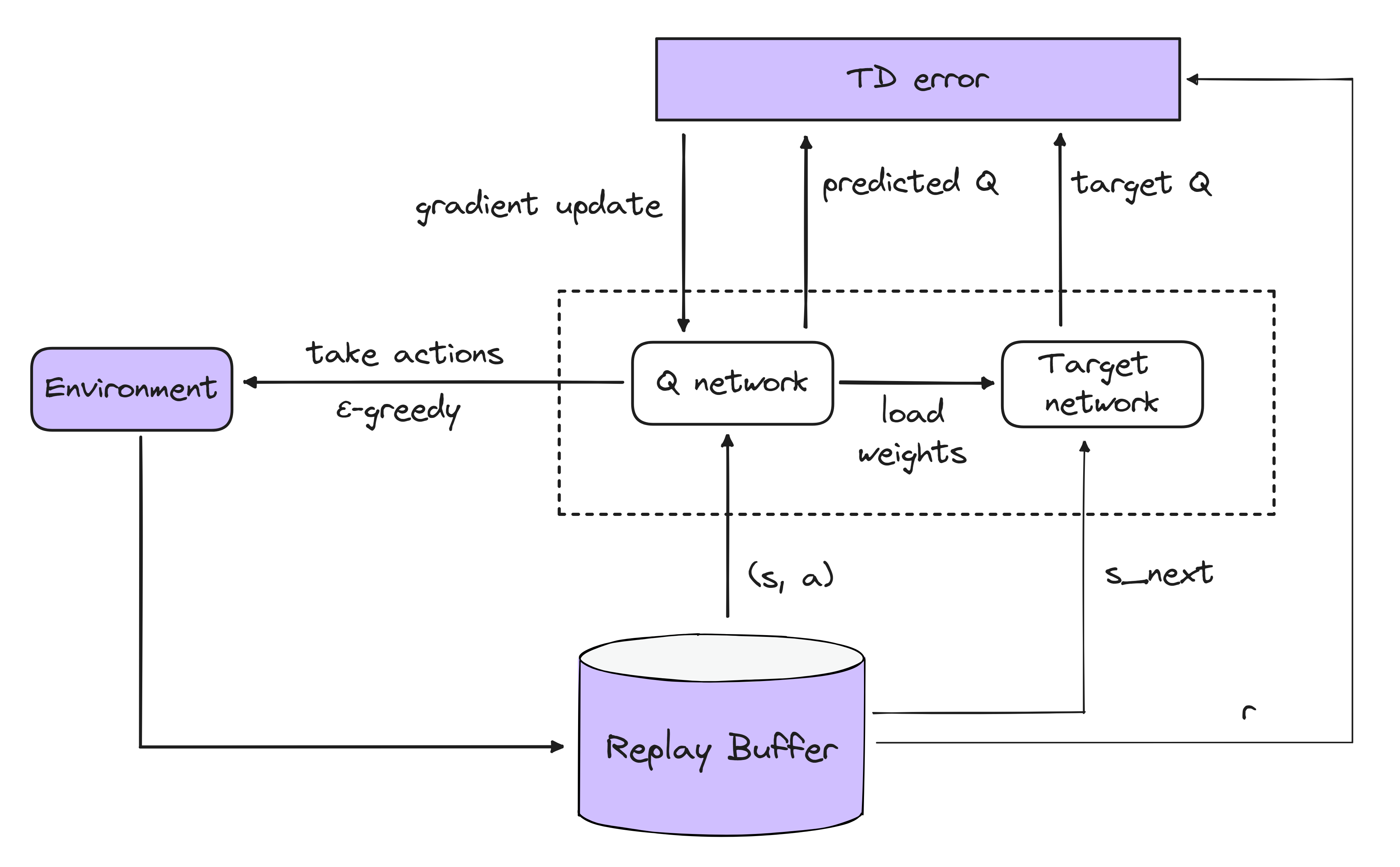
Below is an algorithm showing the conceptual overview of DQN. We cycle through the following process:
- Generate a batch of experiences using our current policy, by epsilon-greedy sampling (i.e. we mostly take the action with the highest Q-value, but occasionally take a random action to encourage exploration). Store these experiences in the replay buffer.
- Use these values to calculate a TD (temporal difference) error, and update our network.
- To increase stability, we also have a target network we use for the "next step" part of the TD error. This is a lagged copy of the Q-network (i.e. we update our Q-network via gradient descent, and then every so often we copy the Q-network weights over to our target network).
- Repeat this until convergence.
Fast Feedback Loops
We want to have faster feedback loops, and learning from Atari pixels doesn't achieve that. It might take 15 minutes per training run to get an agent to do well on Breakout, and that's if your implementation is relatively optimized. Even waiting 5 minutes to learn Pong from pixels is going to limit your ability to iterate, compared to using environments that are as simple as possible.
CartPole
The classic environment "CartPole-v1" is simple to understand, yet hard enough for a RL agent to be interesting, by the end of the day your agent will be able to do this and more! (Click to watch!)
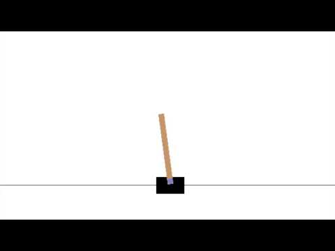
If you'd like to try the CartPole environment yourself, click here to open the simulation in a new tab. * Use Left/Right arrow keys to move the cart, * R to reset, * Q to quit. * Use F/S to make the simulation faster/slower.
Unlike the real CartPole environment, this simulation will not terminate the episode if the pole falls over. We've also cheated here and added a hidden third no-op action, such that if no button is pressed, no force is applied to the cart. This makes the simulation a bit easier for you as the human to play. The real cartpole environment doesn't act like this: the agent must choose to push the cart either left or right on each timestep.
The description of the task is here. Note that unlike the previous environments, the observation here is now continuous. You can see the source for CartPole here; don't worry about the implementation but do read the documentation to understand the format of the actions and observations.
The simple physics involved would be very easy for a model-based algorithm to fit, (this is a common assignment in control theory using proportional-integral-derivative (PID) controllers) but today we're doing it model-free: your agent has no idea that these observations represent positions or velocities, and it has no idea what the laws of physics are. The network has to learn in which direction to bump the cart in response to the current state of the world.
Each environment can have different versions registered to it. By consulting the Gym source you can see that CartPole-v0 and CartPole-v1 are the same environment, except that v1 has longer episodes. Again, a minor change like this can affect what algorithms score well; an agent might consistently survive for 200 steps in an unstable fashion that means it would fall over if run for 500 steps.
We would like to run many copies of this environment in parallel to collect trajectories as fast as possible.
The older way of doing this involved using AsyncVectorEnv
provided by gymnasium, which would spawn num_envs many processes, one for each environment.
This is nice, as it works for an arbitrary environment without any additional effort, but
it doesn't really scale that well. Each process is independent, and each carries their own Python interpreter.
Given that the update rule for the environment itself is trivial,
this overhead is significant. A better approach would be to modify the environment to do the parallelism internally,
spawn a pool of workers and then have threads compute the update rule, but what we do instead is we
port the entire environment dynamics to PyTorch (see chapter2_rl/exercises/gpu_env.py), where
the observations are natively stored as a tensor, and all environments are run in lock-step.
This means * we don't need to constantly convert between numpy and torch tensors, simplifying code * we can run large numbers of environments in parallel (~thousands of environments for ~millions of environmental steps per second) * for toy examples like this where neither the GPU nor the CPU is doing a lot of work, the main bottleneck can just be moving data back and forth between the two.
However, it does add some additional complexity in that it forces all environments to be run for the same number of timesteps, which can cause trouble if some trajectories terminate faster than others. We handle this by allowing the environment to automatically reset upon termination, meaning some rollouts may have more or fewer disjoint episodes, or that an episode may get cut-off halfway.
envs = CartPole(num_envs=4, device=device)

print(envs.single_action_space)  # 2 actions: left and right
print(envs.single_observation_space)  # Box(4): each observation can take a continuous range of values

obs, infos = envs.reset()
print(obs.shape, obs.device)  # (num_envs, 4): one observation per environment, as a tensor on our device
Discrete(2)
Box([-4.8000002e+00 -3.4028235e+38 -4.1887903e-01 -3.4028235e+38], [4.8000002e+00 3.4028235e+38 4.1887903e-01 3.4028235e+38], (4,), float32)
torch.Size([4, 4]) cuda:0
Outline of the Exercises
The exercises are roughly split into 4 sections:
- Implement the Q-network that maps a state to an estimated value for each action.
- Implement a replay buffer to store experiences $e_t = (s_t, a_t, r_{t+1}, d_{t+1}, s_{t+1})$.
- Implement the policy which chooses actions based on the Q-network, plus epsilon greedy randomness to encourage exploration.
- Piece everything together into a training loop and train your agent.
The Q-Network
The Q-Network takes in an observation $s$ and outputs a vector $[Q^*(s, a^1), \ldots Q^*(s,a^n)]$ representing an estimate of the optimal Q-value for the given state $s$, and each possible action $\mathcal{A} = \{a^1, \ldots, a^n\}$. This replaces our Q-value table used in Q-learning.
For best results, the architecture of the Q-network can be customized to each particular problem. For example, the architecture of OpenAI Five used to play DOTA 2 is pretty complex and involves LSTMs.
For learning from pixels, a simple convolutional network and some fully connected layers does quite well. Where we have already processed features here, it's even easier: an MLP of this size should be plenty large for any environment today.
Implement the Q-network using a standard MLP, constructed of alternating Linear and ReLU layers. The size of the input will match the dimensionality of the observation space, and the size of the output will match the number of actions to choose from (associating a reward to each.) The dimensions of the hidden_sizes are provided.
Here is a diagram of what our particular Q-Network will look like for CartPole (you can open it in a new tab if it's hard to see clearly):

Question - why do we not include a ReLU at the end?
If you end with a ReLU, then your network can only predict 0 or positive Q-values. This will cause problems as soon as you encounter an environment with negative rewards, or you try to do some scaling of the rewards.
Question - since CartPole-v1 gives +1 reward on every timestep, why do you think the network doesn't just learn the constant +1 function regardless of observation?
The network is learning Q-values (the sum of all future expected discounted rewards from this state/action pair), not rewards. Correspondingly, once the agent has learned a good policy, the Q-value associated with state action pair (pole is slightly left of vertical, move cart left) should be large, as we would expect a long episode (and correspondingly lots of reward) by taking actions to help to balance the pole. Pairs like (cart near right boundary, move cart right) cause the episode to terminate, and as such the network will learn low Q-values.
Exercise - implement QNetwork
Note - in this implementation we can assume that obs_shape is a tuple of length 1 (in the case of CartPole this will be (4,)), so you can treat it as just an integer value above, e.g. your first linear layer should be from obs_shape[0] to 120.
class QNetwork(nn.Module):
    """
    For consistency with your tests, please wrap your modules in a `nn.Sequential` called `layers`.
    """

    layers: nn.Sequential

    def __init__(self, obs_shape: tuple[int], num_actions: int, hidden_sizes: list[int] = [120, 84]):
        super().__init__()
        assert len(obs_shape) == 1, "Expecting a single vector of observations"
        raise NotImplementedError()

    def forward(self, x: Tensor) -> Tensor:
        return self.layers(x)


net = QNetwork(obs_shape=(4,), num_actions=2)
n_params = sum((p.nelement() for p in net.parameters()))
assert isinstance(getattr(net, "layers", None), nn.Sequential)
print(net)
print(f"Total number of parameters: {n_params}")
print("You should manually verify network is Linear-ReLU-Linear-ReLU-Linear")
assert not isinstance(net.layers[-1], nn.ReLU)
assert n_params == 10934
Solution
class QNetwork(nn.Module):
    """
    For consistency with your tests, please wrap your modules in a `nn.Sequential` called `layers`.
    """

    layers: nn.Sequential

    def __init__(self, obs_shape: tuple[int], num_actions: int, hidden_sizes: list[int] = [120, 84]):
        super().__init__()
        assert len(obs_shape) == 1, "Expecting a single vector of observations"
        in_features_list = [obs_shape[0]] + hidden_sizes
        out_features_list = hidden_sizes + [num_actions]
        layers = []
        for i, (in_features, out_features) in enumerate(zip(in_features_list, out_features_list)):
            layers.append(nn.Linear(in_features, out_features))
            if i < len(in_features_list) - 1:
                layers.append(nn.ReLU())
        self.layers = nn.Sequential(*layers)

    def forward(self, x: Tensor) -> Tensor:
        return self.layers(x)
Replay Buffer
The goal of DQN is to reduce the reinforcement learning problem to a supervised learning problem. In supervised learning, training examples should be drawn identically and independently distributed (i.i.d.) from some distribution, and we hope to generalize to future examples from that distribution. Obviously perfect i.i.d. sampling isn't attainable, but we can approximate this by filling a buffer of past experiences and sampling from it. Note that for very complex problems we may need a very large buffer, because we want the policy to get a representative sample of all the diverse scenarios that can happen in the environment. OpenAI Five used batch sizes of over 2 million experiences for Dota 2! However we'll be working with the fairly simple CartPole environment, and so we can get away with a much smaller buffer.
In RL, the distribution of experiences $e_t = (s_t, a_t, r_{t+1}, s_{t+1})$ to train from depends on the policy $\pi$ followed, which depends on the current state of the Q-value network, so DQN is always chasing a moving target. This is why the training loss curve isn't going to have a nice steady decrease like in supervised learning. We will extend experiences to $e_t = (s_t, a_t, r_{t+1}, s_{t+1}, d_{t+1})$. Here, $d_{t+1}$ is a boolean indicating that $s_{t+1}$ is a terminal observation, and that no further interaction happened beyond $s_{t+1}$ in the episode from which it was generated.
Termination vs Truncation
Note that we take $d_{t+1}$ to be terminated, not done = terminated | truncated. The reason is as follows: our time limit was imposed for practical reasons to help with learning, but if the agent views the environment timing out as a form of failure that terminates its reward then it would have no reason to prefer the behaviour "stay perfectly level" to the behaviour "stay level for the first 499 timesteps then immediately fall over"! We want to encourage the agent to perform well all the time, not just perform well until the environment times out. See this page for more discussion.
We can illustrate this in a bit more depth. Consider the following diagram, which illustrates a set of rollouts from 5 parallel copies of an environment:
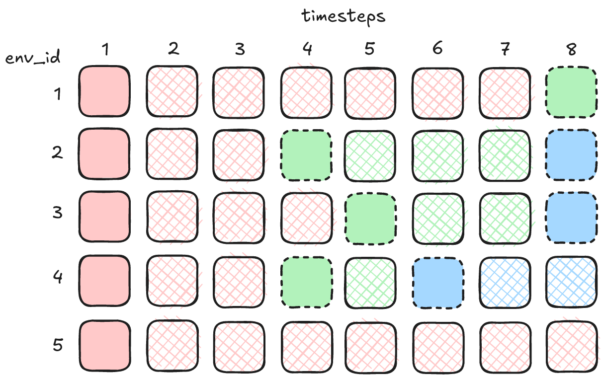
Here, we have 5 parallel environments, each run for 8 timesteps. Different colours denote different episodes. Solid colour denotes the start of each episode, and a dotted border indicates termination occurred during the transition from the previous observation to this one. We can see immediately the (somewhat confusing) convention that when a trajectory terminates, the observation received is the initial observation of the next episode. We can also see the complexity that this poses in the variety of episodes
- Env 1: A single episode that runs for the length of the rollout over 7 timesteps, and terminates on timestep 8.
- Env 2: Two episodes, the first of length 3, which terminates (and on the same timestep we observe the starting state of the second), and the second terminates after 4 timesteps.
- Env 3: The same as Env 2, but the boundary between episodes doesn't match that of Env 2
- Env 4: Three episodes, but the third gets truncated rather than terminated (so the last observation is not drawn with a dotted border)
- Env 5: No episode terminates in time, so the only existing episode gets truncated.
You can see how this might be a problem to handle, especially if it's an environment where you only receive reward at the end of the episode (and zero reward elsewhere). Under these circumstances, Env 5 would give zero feedback at all for learning.
This is why we need the extra code that reads from infos["final_observation"]: given the last
observation $o_T$ for an episode, "$o_{T+1}$" as given from the vectorized environment will be the
starting state of the first episode, but what we actually want to learn from is
the true $o_{T+1}$ (the observation if the environment dynamics act upon $o_t$, ignoring termination).
ReplayBuffer and ReplayBufferSamples
We've given you 2 classes below. The first, ReplayBuffer, holds data from past experiences and also contains methods for sampling that data (the samples are instances of ReplayBufferSamples).
You should read these implementations carefully, making sure you understand how they work. A few things to note:
- The
addmethod adds multiple experiences at once: the tensors likeobshave shape(num_envs, *obs_shape). This is because ourCartPoleis a vectorised environment: a single call toenvs.stepadvances allnum_envsenvironments at once and returns batched tensors, one row per environment. We'll see how this works in practice later. - The
addmethod will add these experiences to the end of the buffer, slicing the buffer if it's too long. Note that the slicing is done so that we remove the oldest experiences when the buffer is full. - The
samplemethod will return aReplayBufferSamplesobject containing the experiences sampled from the buffer. These are sampled with replacement, so the same experience can occasionally appear twice in one batch. That's fine: each draw is still an independent uniform sample from the buffer, so the batch's mean loss is still an unbiased estimate of the mean loss over the whole buffer (and once the buffer is much larger than the batch, duplicates are rare anyway). Everything in the buffer already lives on the GPU as tensors (the environment produces tensors, so there's no numpy anywhere in the loop), which means sampling is just indexing - no data ever has to be copied between the CPU and GPU.
@dataclass
class ReplayBufferSamples:
    """
    Samples from the replay buffer, as PyTorch tensors ready to feed into the Q-network.

    Data is equivalent to (s_t, a_t, r_{t+1}, d_{t+1}, s_{t+1}). Note - here, d_{t+1} is actually **terminated** rather
    than **done** (i.e. it records the times when we went out of bounds, not when the environment timed out).
    """

    obs: Float[Tensor, " sample_size *obs_shape"]
    actions: Int[Tensor, " sample_size"]
    rewards: Float[Tensor, " sample_size"]
    terminated: Bool[Tensor, " sample_size"]
    next_obs: Float[Tensor, " sample_size *obs_shape"]


class ReplayBuffer:
    """
    Contains buffer; has a method to sample from it to return a ReplayBufferSamples object.
    """

    rng: t.Generator
    obs: Float[Tensor, " buffer_size *obs_shape"]
    actions: Int[Tensor, " buffer_size"]
    rewards: Float[Tensor, " buffer_size"]
    terminated: Bool[Tensor, " buffer_size"]
    next_obs: Float[Tensor, " buffer_size *obs_shape"]

    def __init__(
        self,
        num_envs: int,
        obs_shape: tuple[int],
        action_shape: tuple[int],
        buffer_size: int,
        seed: int,
        device: t.device = device,
    ):
        self.num_envs = num_envs
        self.obs_shape = obs_shape
        self.action_shape = action_shape
        self.buffer_size = buffer_size
        self.device = t.device(device)
        self.rng = t.Generator(device=self.device).manual_seed(seed)

        self.obs = t.empty((0, *self.obs_shape), dtype=t.float32, device=self.device)
        self.actions = t.empty((0, *self.action_shape), dtype=t.int64, device=self.device)
        self.rewards = t.empty(0, dtype=t.float32, device=self.device)
        self.terminated = t.empty(0, dtype=t.bool, device=self.device)
        self.next_obs = t.empty((0, *self.obs_shape), dtype=t.float32, device=self.device)

    def add(
        self,
        obs: Float[Tensor, " num_envs *obs_shape"],
        actions: Int[Tensor, " num_envs"],
        rewards: Float[Tensor, " num_envs"],
        terminated: Bool[Tensor, " num_envs"],
        next_obs: Float[Tensor, " num_envs *obs_shape"],
    ) -> None:
        """
        Add a batch of transitions to the replay buffer.
        """
        # Check shapes & datatypes as `t.cat` silently *promotes* dtypes
        for name, data, expected_shape, expected_dtype in zip(
            ["obs", "actions", "rewards", "terminated", "next_obs"],
            [obs, actions, rewards, terminated, next_obs],
            [self.obs_shape, self.action_shape, (), (), self.obs_shape],
            [t.float32, t.int64, t.float32, t.bool, t.float32],
        ):
            assert isinstance(data, Tensor), f"`{name}` should be a tensor, got {type(data)}"
            assert data.shape == (self.num_envs, *expected_shape), f"`{name}` has shape {tuple(data.shape)}, expected {(self.num_envs, *expected_shape)}"
            assert data.dtype == expected_dtype, f"`{name}` has dtype {data.dtype}, expected {expected_dtype}"

        # Add data to buffer, slicing off the old elements
        self.obs = t.cat((self.obs, obs))[-self.buffer_size :]
        self.actions = t.cat((self.actions, actions))[-self.buffer_size :]
        self.rewards = t.cat((self.rewards, rewards))[-self.buffer_size :]
        self.terminated = t.cat((self.terminated, terminated))[-self.buffer_size :]
        self.next_obs = t.cat((self.next_obs, next_obs))[-self.buffer_size :]

    def sample(self, sample_size: int) -> ReplayBufferSamples:
        """
        Sample a batch of transitions from the buffer, with replacement.
        """
        # Independent uniform draws, so duplicates are possible
        indices = t.randint(0, self.obs.shape[0], (sample_size,), generator=self.rng, device=self.device)

        return ReplayBufferSamples(
            obs=self.obs[indices],                  # s_t
            actions=self.actions[indices],          # a_t
            rewards=self.rewards[indices],          # r_{t+1}
            terminated=self.terminated[indices],    # d_{t+1}: terminated (not truncated!)
            next_obs=self.next_obs[indices],        # s_{t+1}
        )
Next, you can run the following code to visualize your cart's position and angle, and see how these look in both the buffer and the buffer's random samples. Do the samples look correctly shuffled? Also, based on the CartPole source code, do the angles & positions at which the cart terminates make sense? (Note, the min/max values in the table are different to the termination ranges, the latter can be found below the table in the docstring.)
Note that the code below uses our batched CartPole with num_envs=1, so every tensor it returns has a leading dummy batch dimension of size 1 (one row per environment).
Lastly, note how when we terminate environments we do something slightly different. If envs.step results in some environments terminating, it'll actually return next_obs as the reset observation for the next episode. In this case, we want to use this as our starting observation for the next step, but we need to make sure we record the correct terminal observation in our buffer - we do this by extracting it from the infos dict, which is where it gets stored. You can see this in the plots below: the vertical lines are the values $t$ where $d_{t+1}=1$ i.e. $s_{t+1}$ is terminal, and we can see that $s_t$ is the final observation of the terminated episode while $s_{t+1}$ is the first observation of the new episode immediately after.
buffer = ReplayBuffer(num_envs=1, obs_shape=(4,), action_shape=(), buffer_size=256, seed=0, device=device)
envs = CartPole(num_envs=1, seed=0, device=device)
obs, infos = envs.reset()

for i in range(256):
    # Choose random actions (one per environment), and take a step in the environment
    actions = t.randint(0, envs.single_action_space.n, (envs.num_envs,), device=device)
    next_obs, rewards, terminated, truncated, infos = envs.step(actions)

    # Get `true_next_obs` by finding all environments where we terminated & replacing `next_obs`
    # with the actual terminal states (the env has already auto-reset those environments, and stored
    # the observation they ended on in `infos["final_observation"]`)
    done = terminated | truncated
    true_next_obs = next_obs.clone()
    true_next_obs[done] = infos["final_observation"][done]

    # Add experience to buffer
    buffer.add(obs, actions, rewards, terminated, true_next_obs)
    obs = next_obs

sample = buffer.sample(256)

plot_cartpole_obs_and_dones(
    buffer.obs.cpu(),
    buffer.terminated.cpu(),
    title="Current obs s<sub>t</sub><br>so when d<sub>t+1</sub> = 1, these are the states just before termination",
)

plot_cartpole_obs_and_dones(
    buffer.next_obs.cpu(),
    buffer.terminated.cpu(),
    title="Next obs s<sub>t+1</sub><br>so when d<sub>t+1</sub> = 1, these are the terminated states",
)

plot_cartpole_obs_and_dones(
    sample.obs.cpu(),
    sample.terminated.cpu(),
    title="Current obs s<sub>t</sub> (sampled)<br>this is what gets fed into our model for training",
)