3️⃣ Explaining the Vectorized MCTS
Learning Objectives
- Understand how we can restructure the sequential version to batch the
evaluatestage of the MCTS algorithm.- Understand both Root Parallelization and Leaf Parallelization, how they work, and why Root Parallelization is suited for implementing in PyTorch.
- Build a simulated version of Root Parallelization that uses the sequential version as the backend.
Your single-game MCTS is correct but slow: one network call per simulation, on a single board. A GPU wants big batches. To train in minutes we need to run hundreds of self-play games at once, with every per-simulation network call batched into one forward pass.
Root Parallelism (we do this)
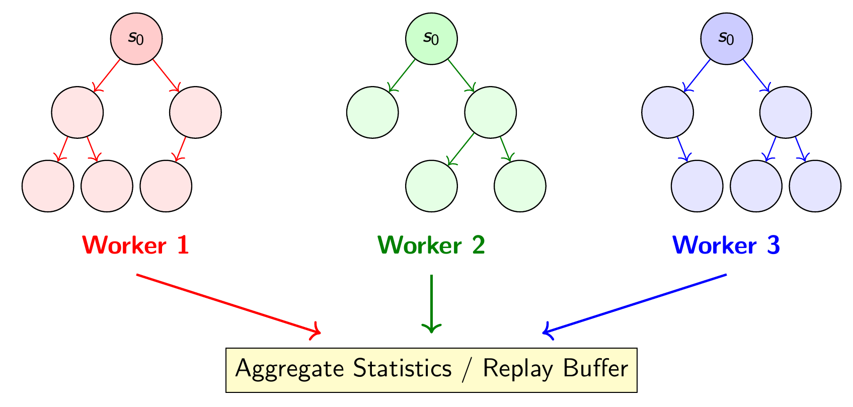
We run batch_size independent games, each with its own search tree. The trees never interact.
We batch them purely for GPU throughput: after all workers have finished selection and expansion,
we collect all the nodes together and do a single forward pass throguh the network to evaluate all
the leaves in one go. All trees then backup the values to their respective roots.
After the MCTS search is done, from each tree $T_i$ we derive a respective tree policy $\pi_i$, and
we sample an action from each to get a set of batch_size many actions,
and then step all batch_size many environment by one timestep.
During the training phase, we collect data $(z,s, \pi)$ from all of the enviromental rollouts, and train the actor/critic network according to the loss mentioned earlier:
The fact that all trees share the same network is the only mechanism by which the trees can causally effect each other.
What gives us the sheer speed is that everything runs on the GPU:
* All of the trees, as well as the operations on them are written as vectorized operations on the GPU. Each operation
(walking down or up the tree, updating nodes) are all performed in lockstep, so there is no need to synchronize between threads.
The downside of this approach is the additional complication that not all leaf nodes will be at the same depth, nor do all games run
for the same number of steps. We will see how to handle this.
* The environment itself is vectorized, we can easily run many thousands of games in parallel, and the rules for updating
the game state, or checking for a winner, are all written as vectorized PyTorch operations (e.g. the operation of checking for a 4-in-a-row can be written as a convolution using kernels with hardcoded weights, see game.py)
At no point do we need to copy any data back and forth between the CPU or the GPU, as all the data is generated by interaction with the environment, and for a game like Connect-4, the state space is relatively small, and the length of the games reasonably bounded, so the memory usage is not a concern. Expect effectively ~millions of environment steps per second during training (the environment itself can run at tens-of-millions of steps per second before the rules of the game are the bottleneck).
Tree Parallelism (too complex for us)
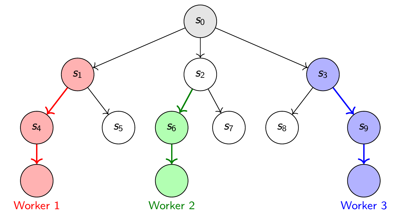
We could have used one shared tree with many workers descending it simultaneously. It can be more sample-efficient as all workers pool their statistics into one tree, whereas root parallelism can be wasteful and have differnet trees generate duplicate statistics. But we have a different problem: Several workers running up and down the tree to update nodes leads to node contention: workers may have to wait for a node to be free while another worker is updating it, else we may read out a stale value, or worse, overwrite another worker's updates.
This can be solved with mutexes: when a worker wants to write to a node, it first locks it so no other worker can, reads the value, processes it, and then writes back the new value. With several workers waiting for the same node (e.g. the root node), this can the gains one hoped to get from tree parallelism. It also means you could hash the board state before expanding to see if the node already exists somewhere else, and then jump there instead. This means your MCTS search is operating over a DAG (directed acyclic graph) instead of a tree, leading to some complications on keeping track of the path from a given leaf to the root node. This is a nightmare to write vectorized on the GPU (trust me, I tried!), you would instead write the tree updating code in highly optimized C++, and then have data shuffled back and forth between the CPU and the GPU when you want to query the network (this was also a nightmare when I tried it).
Leaf Parallelism is (to the best of my knowedge) the method that DeepMind used for AlphaZero, but we use root parallelism instead as it's much easier to implement as vectorized code on the GPU, and the speed gains from having everything be on the GPU outweigh the cost of several trees duplicating work.
Root exploration noise (given)
Self-play has a chicken-and-egg problem: MCTS is steered by the network's prior, so it mostly explores moves the network already likes — and the network only learns about moves the search explores. A young network can collapse onto a narrow set of openings and never discover better ones.
AlphaZero's fix is to add Dirichlet noise to the prior at the root only — never inside the tree, so it changes which lines get explored without corrupting the search's own value estimates:
The Dirichlet distribution is a distribution over probability vectors $\eta=(\eta_1,\dots,\eta_n)$ with $\eta_i \ge 0$ and $\sum_i \eta_i = 1$ i.e. over the probability simplex. In general it has one concentration parameter per component, $\alpha_1,\dots,\alpha_n$, but we use the same $\alpha$ for all of them (a symmetric Dirichlet). That single $\alpha$ controls how spiky the samples are:
- $\alpha < 1$: spiky / sparse: most weight lands on one or two moves, so the noise occasionally gives a normally-ignored column a big boost (strong, targeted exploration).
- $\alpha = 1$: uniform over the simplex.
- $\alpha > 1$: flat: close to the centroid $(1/n,\dots,1/n)$, only a mild perturbation.
The plot below shows the Dirichlet density on the $n=3$ simplex (a triangle, one corner per
component); drag the $\alpha$ slider (log scale) to watch the mass move between the corners (spiky)
and the centre (flat). dirichlet_root_noise is given:
def dirichlet_root_noise(
    prior: Float[Tensor, "... 7"],
    legal: Bool[Tensor, "... 7"],
    alpha: float,
    eps: float,
) -> Float[Tensor, "... 7"]:
    """Mix Dirichlet exploration noise into the root prior (used by `expand_root` when `add_noise`).

    Noise is added only at the root, which keeps self-play exploring without distorting the rest of
    the tree. `eps = 0` returns `prior` unchanged. We use a symmetric Dirichlet (the same `alpha`
    for every column). Works with or without a leading batch dimension.

    Args:
        prior: (..., 7) the network prior at the root
        legal: (..., 7) legal-column mask (the noise is renormalised over the legal columns)
        alpha: Dirichlet concentration (smaller = spikier noise)
        eps:   mixing weight on the noise

    Returns:
        (..., 7) the mixed prior `(1 - eps) * prior + eps * noise`
    """
    noise = torch.distributions.Dirichlet(
        torch.full((prior.shape[-1],), alpha, device=prior.device)
    ).sample(prior.shape[:-1])
    noise = noise * legal.float()
    noise = noise / noise.sum(-1, keepdim=True).clamp_min(1e-8)
    return (1.0 - eps) * prior + eps * noise


tests.test_dirichlet_root_noise(dirichlet_root_noise)
To plot the Dirichlet density on the 3-simplex; drag the alpha slider (log scale, 0.01 -> 10).
utils.plot_dirichlet_simplex()
A stepping stone: batch the network, keep the Python trees
Before we rewrite everything as vectorised tensor ops, here's a much gentler version that already captures the two ideas that make root parallelism fast:
We keep num_env completely independent single-game trees, each built from the exact primitives
(select, expand, backup). Per MCTS simulation we:
- select + expand each tree, sequentially with a plain Python
forloop, collecting one leaf node per tree (pretending they run in parallel); - evaluate all
num_envleaves in a single fixed-size forward pass through the network; - backup each tree, again sequentially with a
forloop (pretending they run in parallel).
In principle both loops could be accelerated by dispatching multiple threads:
from concurrent.futures import ProcessPoolExecutor

#each piece of data processed individually by `work`
def work(x):
    ...
    return something

data = [1, 2, 3, 4, 5]
with ProcessPoolExecutor() as ex:
    results = list(ex.map(work, data))
but the overhead of dispatching threads, and copying data CPU <-> GPU would kill us.
Two details bring it closer to the real vectorised search:
- A shared obs pool. Rather than every node owning its own
(1, 3, H, W)board, we keep oneobs_pooltensor of shape(B, MAXN, 3, H, W)and each node just stores an integerslotpointing into it. The root boards go in once (obs_pool[:, 0] = root_obs); the per-simulation batch is then a single gather out of the pool, with no packing/unpacking. This is exactly the storage scheme of the vectorisedTreebelow. - A fixed-size batch. We push all
Bleaves through the network every simulation, including terminal ones whose value we already know. Re-evaluating a terminal leaf is wasted compute, but a constantB-shaped forward pass every step is both faster on the GPU and faithful to the vectorised search, where the batch shape never changes. This also works better withtorch.compilefor extra speed.
The gains are minimal (I measured ~1.8x speed-up against the purely sequential version), but it's a good starting point.
class SimulatedBatchedMCTS:
    """Root-parallel MCTS over `B` independent trees, with the network call batched across trees.

    A clarity-first stand-in for the vectorised `BatchedMCTS` below, with the **same interface**: hold
    an `env` + `cfg`, then call `.search(model, root_obs, root_is_player1)`. Every tree is a normal
    Python `Node` tree driven by the section 2 `select`/`backup` functions, looped over the batch. The two
    things it borrows from the vectorised version are (i) a single `obs_pool` that every node indexes
    by `slot` (so boards never need packing/unpacking), and (ii) a fixed-size forward pass over all
    `B` leaves every simulation, terminal leaves included.

    Each node stores an integer `slot` instead of its own board: its position lives at
    `obs_pool[game, slot]`. (`Node.obs` is left as `None` since none of `select`/`backup` read it.)
    """

    def __init__(self, env, cfg):
        self.env, self.cfg = env, cfg

    @torch.no_grad()
    def _expand(self, obs_pool, nptr, game, node, action):
        """Section 2's `expand` function, but the child's board is written into the pool and the child stores its `slot`."""
        parent_obs = obs_pool[game, node.slot].unsqueeze(0)                 # (1, 3, H, W) view into pool
        next_obs, done, reward = self.env.step(parent_obs, action, node.is_player1)
        slot = nptr[game]
        nptr[game] += 1
        obs_pool[game, slot] = next_obs[0]
        child = Node(obs=None, is_player1=~node.is_player1, is_terminal=done,
                     terminal_value=-reward, parent=node, parent_action=action)
        child.slot = slot
        node.children[action] = child
        return child

    @torch.no_grad()
    def _evaluate_batch(self, model, obs_pool, batch_idx, nodes):
        """Evaluate all `B` leaves in ONE fixed-size forward pass; return one value per node.

        Terminal leaves are forwarded too (their board is gathered from the pool like any other) even
        though we throw away the network's output and use the value stored at creation. The constant
        `B`-shaped batch matches the vectorised search and is faster than a ragged one.
        """
        slots = torch.tensor([node.slot for node in nodes], device=obs_pool.device)
        obs = obs_pool[batch_idx, slots]                                   # (B, 3, H, W), one gather
        is_player1 = torch.cat([node.is_player1 for node in nodes])        # (B,)
        value, logits = eval_net(model, obs, is_player1)                   # <- one batched call, all B nodes
        value, logits = value.cpu(), logits.cpu()
        legal = self.env.legal_action_mask(obs).cpu()
        P = torch.softmax(torch.where(legal, logits, -torch.inf), dim=-1)
        values = []
        for b, node in enumerate(nodes):
            if node.is_terminal:
                values.append(node.terminal_value)    # value known at creation; net output discarded
            else:
                node.legal = legal[b]
                node.P = P[b]
                values.append(float(value[b]))
        return values

    @torch.no_grad()
    def search(self, model, root_obs: Float[Tensor, "B 3 6 7"], root_is_player1: Bool[Tensor, "B"],
               add_noise: bool = False) -> Float[Tensor, "B 7"]:
        """Run `cfg.sims` simulations of root-parallel MCTS; return (B, 7) root visit counts.
        Same signature as `BatchedMCTS.search`, just sequential-over-trees (so much slower)."""
        cfg = self.cfg
        B, device = root_obs.shape[0], root_obs.device
        batch_idx = torch.arange(B, device=device)

        # Shared obs pool: every node just stores a `slot` into this, so we never pack/unpack boards.
        # At most one node is added per simulation, so `cfg.sims + 1` slots per game (slot 0 = root)
        # can never overflow.
        obs_pool = torch.zeros((B, cfg.sims + 1, *root_obs.shape[1:]), dtype=root_obs.dtype, device=device)
        obs_pool[:, 0] = root_obs                    # drop in all root boards at once (slot 0)
        nptr = [1] * B                               # next free slot per game

        # construct the roots of the trees, each pointing at slot 0 of its game's pool
        roots = []
        for b in range(B):
            node = Node(obs=None, is_player1=root_is_player1[b].unsqueeze(0))
            node.slot = 0
            roots.append(node)

        # evaluate every root in one forward pass to set its P / legal (as section 2 does for its single root)
        self._evaluate_batch(model, obs_pool, batch_idx, roots)
        if add_noise:  # batched Dirichlet noise on the root priors, exactly as `expand_root` does it
            P = dirichlet_root_noise(torch.stack([r.P for r in roots]), torch.stack([r.legal for r in roots]),
                                     cfg.dirichlet_alpha, cfg.dirichlet_eps)
            for b, root in enumerate(roots):
                root.P = P[b]

        for _ in range(cfg.sims):
            # 1. SELECT + EXPAND each tree sequentially, collecting one leaf per tree
            leaves = []
            for game, root in enumerate(roots):
                node, action = select(root, cfg.c_puct)
                leaf = node if node.is_terminal else self._expand(obs_pool, nptr, game, node, action)
                leaves.append(leaf)
            # 2. EVALUATE every leaf in a single, fixed-size forward pass through the network
            values = self._evaluate_batch(model, obs_pool, batch_idx, leaves)
            # 3. BACKUP each tree sequentially
            for leaf, value in zip(leaves, values):
                backup(leaf, value)
        return torch.stack([root.N for root in roots]).to(device)      # (B, 7), on the input's device

tests.test_simulated_batched_mcts(SimulatedBatchedMCTS)
Unsurprisingly, this barely helps, as the largest bottleneck is just looping through all the tree updates:
benchmarking this against the fully-accelerated version below (sims=32, NVIDIA RTX A4000, 16GB RAM):
| B | seq-trees + batched-net | batched-everything | speedup | GPU Mem |
|---|---|---|---|---|
| 64 | 716 | 4,751 | 6.6× | nil |
| 256 | 704 | 19,572 | 28.8× | nil |
| 1,024 | 689 | 78,325 | 114× | 0.12 GB |
| 4,096 | 691 | 189,903 | 275× | 0.44GB |
| 8,192 | 700* | 208,591 | 298× | 0.86 GB |
| 16,384 | 700* | 220,152 | 314× | 1.71 GB |
| 32,768 | 700* | 226,132 | 323× | 3.41 GB |
| 65,536 | 700* | 229,872 | 328× | 6.80 GB |
| 131,072 | 700* | OOM | - | > 16 GB |
*Estimated based on the average over lower batches as it took too long to run, and that we don't expect larger batch sizes to help the sequential version anyway.
As we can see, the seqential version is flat at ~700 env-steps/s even with small batch sizes, as processing the trees is by far the bottleneck. Once we vectorize everything, it saturates at roughly ~220k env-steps/s, a 300x speedup.
For now, we will take for granted the vectorized implementation of MCTS, which provides
a functionally identical BatchedMCTS.search method as SimulatedBatchedMCTS.search above,
but implemented such that selection, expansion and backup are
also vectorized.
As a bonus at the end you can try implementing the vectorized version yourself.