0️⃣ MCTS & AlphaZero — Theory
Learning Objectives
- Understand the four phases of MCTS (selection, expansion, simulation, backup).
- See how AlphaZero replaces random rollouts with a value net and uses the policy as a prior via PUCT.
- Understand the self-play loop and loss function for the network.
Vanilla Monte Carlo Tree Search
Connect 4 is a two-player, perfect-information, zero-sum game on a 6×7 grid. Our goal is an agent that learns strong play from self-play alone. It is a strongly solved game: the optimal move is known from any board position, while still being a challenging game to play optimally. This is useful as we have ground truth values with which our agent can be measured against.
Vanilla MCTS
Each node stores visit counts $N$, value sums $W$, and pointers to it's children. The nodes represent states of the game, and the edges represent actions taken to transition between states.
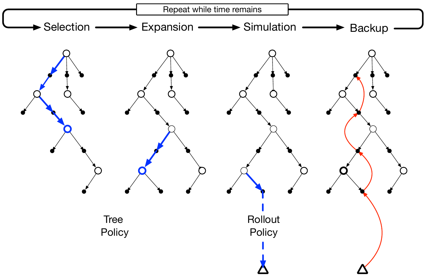
Monte Carlo Tree Search builds a search tree rooted at the current position by repeating four phases, many times:
- Selection. Starting at the root, repeatedly pick a child according to a tree policy that balances exploiting good moves and exploring uncertain ones, until you reach a leaf node.
- Expansion. Add a new child to the leaf node.
- Simulation (rollout). From the new node, simulate both players with random moves until the end of the game and observe who won.
- Backup. Propagate the result back up the path, incrementing visit counts $N$ and value sums $W$ at every node on the way.
After iterating, the most-visited move at the root is the actual action the agent chooses to play.
From MCTS to AlphaZero
AlphaZero keeps the tree-search skeleton but makes two changes. First, we define a neural network $f_\theta$ with parameters $\theta$, mapping a state $s \in \mathcal{S}$ to a pair $(\mathbf{p}, v)$:
- The policy $\mathbf{p}(\cdot | s) \in \Delta(\mathcal{A})$ is a probability distribution over actions — $\Delta(\mathcal{A})$ denotes the set of all probability distributions over the action set $\mathcal{A}$, i.e. for Connect 4 a vector of 7 non-negative numbers summing to 1. It acts as a prior over which moves look promising, before any search is done.
- The value $v(s) \in [-1, 1]$ is an estimate of the game's eventual outcome, from the perspective of the player about to move ($-1$ = certain loss, $+1$ = certain win).
With this network, the changes to MCTS are:
-
No random rollouts. From leaf node $s$, we directly query the critic head $v(s)$ to get an estimate of the game's outcome (or if the game has ended, the ground-truth reward $z \in \{-1, 0, +1\}$ for loss/draw/win respectively).
-
A policy prior in selection. We use PUCT (Predictor + Upper Confidence Trees), which biases exploration toward moves the policy likes:
$$ PUCT(s,a) = \underbrace{Q(s, a)}_{\text{exploitation}} + \underbrace{c \cdot p_\theta(a|s) \cdot \frac{\sqrt{1 + \sum_{a'} N(s,a')}}{1 + N(s, a)}}_{\text{exploration}} $$
The terms are statistics stored on the tree's edges and updated during backup:
- $N(s, a)$ is the visit count: how many simulations have taken action $a$ from state $s$ so far. Summing over the actions, $N(s) := \sum_{a'} N(s,a')$, gives the total number of visits to $s$ itself.
- $W(s, a)$ is the total value: the sum of all backed-up outcomes (value estimates $v$, or terminal rewards $z$) from simulations that took action $a$ from state $s$.
- $Q(s, a) := W(s,a) / \max(1, N(s,a))$ is the mean value: the empirical average outcome of taking $a$ from $s$. This is the exploitation term — it is high for moves that have done well in the search so far.
- $p_\theta(a|s)$ is the policy head's prior probability for action $a$ in state $s$, before any search.
- $c$ is a hyperparameter trading off exploitation ($Q$) against exploration (the prior-weighted second term).
The exploration term is large when $a$ has a high prior but few visits relative to its siblings, and it shrinks as $N(s,a)$ grows — so the search initially follows the policy's suggestions, then increasingly trusts the values it has actually measured.
Why $\sqrt{1 + \sum_b N(b)}$ rather than $\sqrt{\sum_b N(b)}$?
It matters only on a node's first visit, when every $N(b) = 0$. Then $Q = 0$ and, with a bare $\sqrt{\sum N} = 0$, every legal action scores $0$ — so
argmaxjust picks the first legal column and ignores the policy. The $+1$ makes $PUCT(s,a) \propto p_\theta(a|s)$ on that first visit, so the search follows the prior straight away, which can help if doing very few MCTS iterations. Doesn't make much of a difference for large numbers of simulations.
Why $z$ for reward?
Dunno. That was the notation used in the original AlphaZero paper.
Interactive: watch MCTS think
Here's a small interactive visualiser (standalone JavaScript, runs in your browser). Set up a Connect-4 position, run the search, then you can step through the simulations to watch the tree grow node-by-node, with each node's visit count $N$, mean value $Q$ and prior $P$. This is the four-phase MCTS loop (select → expand → simulate → back-up) which is run once per simulation.
▶ Open the interactive MCTS visualiser (new tab)
The self-play training loop
Each move of a self-play game:
- Generate a node representing the current position of the game, and run the network to obtain an estimate $v(s)$ of the games outcome, as well as a prior $p_\theta(\cdot|s)$ for the actions to take from this position.
-
Optionally, for the root node only, we inject Dirichlet noise into the prior to encourage exploration.
-
Run several simulations of MCTS from the current position:
- Selection: Starting at the root, walk down the tree following the PUCT selection policy.
$$ \pi^\text{PUCT}(s) = \arg\max_{a} PUCT(s, a) $$until you run out of nodes to explore (or the node is terminal because the game ended).
- Expansion: If the node is not terminal, add a new child node to the leaf node.
- Evaluation: If the node is not terminal, evaluate the new child node using the critic network $v(s)$ to get an estimate of the game's outcome (or, if the child is terminal, the ground-truth reward $z \in \{-1, 0, +1\}$ for loss/draw/win respectively).
- Backup: Propagate the result back up the path, incrementing visit counts $N$ and value sums $W$ at every node on the way.
- Selection: Starting at the root, walk down the tree following the PUCT selection policy.
-
The normalised visit counts
$$ \pi(a | s) := \frac{N(s, a)^{1/\tau}}{\sum_{a'} N(s, a')^{1/\tau}} $$are the target policy: a policy improved by tree search that should give better moves than the raw policy network $p_\theta$. -
Sample the actual move from $\pi$ (with temperature $\tau$ for exploration). During training, $\tau = 1$ to encourage exploration ($\pi(a|s) \propto N(a,s)$) and during evaluation, we send $\tau \to 0$, which causes $\pi$ to sample the action $a$ with the highest visit count $N(a,s)$
$$ \pi(a|s)\big|_{\tau \to 0} = \begin{cases} 1 & \text{if } a = \arg\max_{a'} N(s, a') \\ 0 & \text{otherwise} \end{cases} $$ -
We train the network to try and predict the target policy, and we train the critic to predict the value of the position.
$$ \mathcal{L}(\theta) = \mathbb{E}_{s,z,\pi \sim \mathcal{D}} \left[ (z - v(s))^2 - \sum_{a} \pi(a|s) \log p_\theta(a|s) \right] + c ||\theta||^2 $$where -
$z$ are the ground truth reward based on the outcome of a game (win = 1, draw = 0, loss = -1),
- $s$ are the states of the game visited during rollouts, and
- $\pi(\cdot | s)$ are the tree policies for those states
So, what is the data distribution $\mathcal{D}$ that we are sampling from? It is the distribution of states, rewards, and tree policies obtained from rollouts from self-play (the network plays games against itself).
What about the terms in the loss function?
- The term $(z - v(s))^2$ trains the critic $v$ to try and predic the ground truth reward $z$ for the position $s$.
- The term $-\sum_{a} \pi(a|s) \log p_\theta(a|s)$ is standard cross-entropy loss to try and train the network $p_\theta$ to act like the tree policy $\pi$. The tree policy uses the network + planning via the MCTS tree, so we expect that $\pi$ to be stronger than $p_\theta$. By training the network to act like the tree policy, we are trying to distill the planning process into the network itself (which in turn gives a stronger tree policy, and so on).
- The term $c ||\theta||^2$ is just a standard reguliarization term to prevent the network from overfitting. In practice, I found the network trains just fine without it, but it's included here for completeness as it was present in the original AlphaZero paper.
You'll note that this is a very strange loss function for RL, and is wholly unlike policy gradient methods. This can almost be seen as a kind of distillation loss where we are trying to teach $p_\theta$, the student model, to act like $\pi$, the teacher model, except the teacher itself is bootstrapped from the student itself, plus the performance boost given by MCTS. We will see an example later on of how, every with a randomly initalized $p_\theta$, $\pi$ is still notably stronger, giving $p_\theta$ something to latch onto and improve itself.