1️⃣ GANs
Learning Objectives
- Understand the loss function used in GANs, and why it can be expected to result in the generator producing realistic outputs.
- Implement the DCGAN architecture from the paper, with relatively minimal guidance.
- Learn how to identify and fix bugs in your GAN architecture, to improve convergence properties.
Reading
- Google Machine Learning Education, Generative Adversarial Networks (strongly recommended, ~15 mins)
- This is a very accessible introduction to the core ideas behind GANs
- You should read at least the sections in Overview, and the sections in GAN Anatomy up to and including Loss Functions
- Unsupervised representation learning with deep convolutional generative adversarial networks (optional, we'll be going through parts of this paper later on in the exercises)
- This paper introduced the DCGAN, and describes an architecture very close to the one we'll be building today.
- It's one of the most cited ML papers of all time!
Loading data
We'll be training on the Celeb-A dataset (a large-scale dataset of more than 200k celebrity faces), and optionally on MNIST. Both are loaded with get_dataset from fundamentals_utils, exactly as in the VAEs section: see Loading data there for how these datasets work (in particular, that they yield raw uint8 images, and your training loop applies trainset.transform after moving each batch to the device).
The first call downloads Celeb-A into HuggingFace's cache, which can take a few minutes, so you might want to run the cell below before you start the reading.
trainset_celeb = get_dataset("CELEB")
x = next(iter(DataLoader(trainset_celeb, batch_size=25)))[0]
display_data(trainset_celeb.transform(x), nrows=5, title="CelebA data")
How GANs work
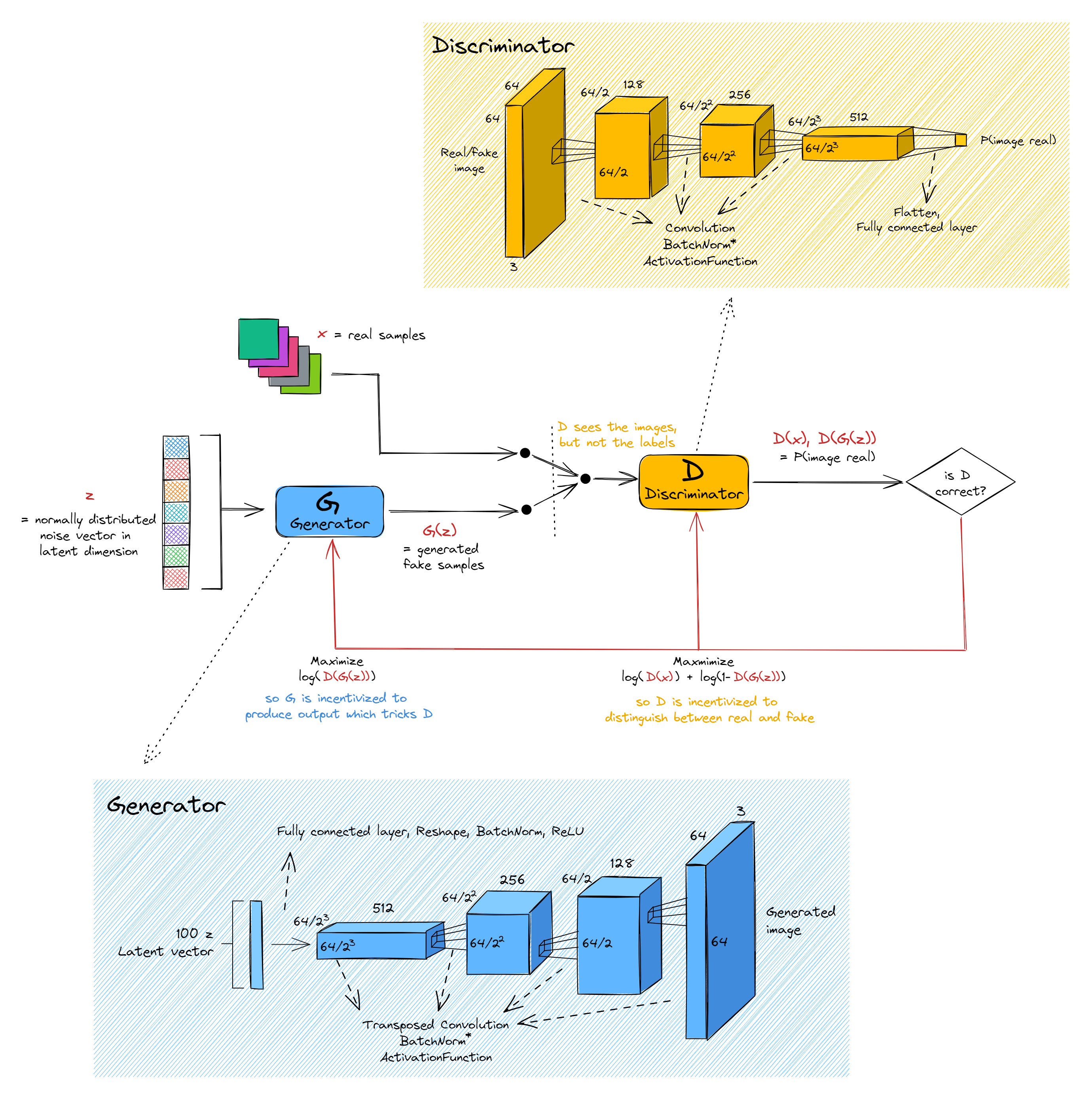
The basic idea behind GANs is as follows:
- You have two networks, the generator and the discriminator.
- The discriminator's job is to distinguish reality from fiction by classifying images as either real from the dataset, or fake from the generator.
- The generator's job is to generate images that fool the discriminator into classifying them as real.
Both networks are trained simultaneously, in a positive feedback loop: as the generator produces better output, the discriminator's job becomes harder, and it has to learn to spot more subtle features distinguishing real and fake images, meaning the generator has to work harder to produce images with those features, and so on. What we'd like at the end of training is for the generator to win, and produce images that look so realistic that the discriminator is no better than random guessing.
Discriminator
The discriminator works by taking an image (either real, or created by the generator), and outputting a single value between 0 and 1, which is the probability that the discriminator puts on the image being real. It is simply a binary classifier, with the loss function being cross entropy between its probability estimates ($D(x)$ for real images, $D(G(\mathbf{z}))$ for fake images) and the true labels ($1$ for real images, $0$ for fake images).
Generator
The architecture of generators in a GAN setup is generally a mirror image of the discriminator, with convolutions swapped out for transposed convolutions. This is the case for the DCGAN paper we'll be reading (which is why they only give a diagram of the generator, not both). The generator works by taking in a vector $\mathbf{z} \sim \mathcal{N}(\mathbf{0}, \mathbf{I})$, whose elements are all normally distributed with mean 0 and variance 1. We call the space from which $\mathbf{z}$ is sampled latent dimension or latent space, and we call a particular $\mathbf{z}$ a latent vector. The formal definition of a latent space is an abstract multi-dimensional space that encodes a meaningful internal representation of externally observed events. We'll dive a little deeper into what this means and the overall significance of latent spaces later on, but for now it's fine to understand this vector $\mathbf{z}$ as a kind of random seed, which causes the generator to produce different outputs. After all, if the generator only ever produced the same image as output then the discriminator's job would be pretty easy: it would just memorise the image the generator produces (no matter how realistic it may seem) and classify it as fake. The generator's objective function is an increasing function of $D(G(\mathbf{z}))$, in other words it tries to produce images $G(\mathbf{z})$ which have a high chance of fooling the discriminator (i.e. ideally $D(G(\mathbf{z})) \to 1$).
Convergence
The ideal outcome when training a GAN is for the generator to produce perfect output indistinguishable from real images, and the discriminator just guesses randomly. However, the precise nature of the situations when GANs converge is an ongoing area of study (in general, adversarial networks have very unstable training patterns). For example, you can imagine a situation where the discriminator becomes almost perfect at spotting fake outputs, because of some feature that the discriminator spots and that the generator fails to capture in its outputs, or if the generator always generates images with some flaw that the discriminator learns. It will be very difficult for the generator to get a training signal, because it has to figure out what feature is missing/present from its outputs, and how it can add/remove that feature to fool the discriminator. To make matters worse, maybe marginal steps in that direction will only increase the probability of fooling the discriminator from almost-zero to slightly-more-than-almost-zero, which isn't much of a training signal! Later on we will see techniques people have developed to overcome problems like this and others, but in general they can't be solved completely, and adversarial training dynamics are just unstable and messy in general.
Optional exercise - what conditions must hold for the discriminator's best strategy to be random guessing with probability 0.5?
It is necessary for the generator to be producing perfect outputs, because otherwise the discriminator could do better than random guessing.
If the generator is producing perfect outputs, then the discriminator never has any ability to distinguish real from fake images, so it has no information. Its job is to minimise the cross entropy between its output distribution $(D(x), 1-D(x))$, and the distribution of real/fake images. Call this $(p, 1-p)$, i.e. $p$ stands for the proportion of images in training which are real. Note how we just used $p$ rather than $p(x)$, because there's no information in the image $x$ which indicates whether it is real or fake. Trying to minimize the cross entropy between $(p, 1-p)$ and $(D(x), 1-D(x))$ gives us the solution $D(x) = p$ for all $x$. In other words, our discriminator guesses real/fake randomly with probability equal to the true underlying frequency of real/fake images in the data. This is 0.5 if and only if the data contains an equal number of real and fake images. We force this to be the case during training, so the discriminator can't simply always guess the class that has the highest frequency.
To summarize, the necessary and sufficient conditions for $(\forall x) \; D(x) = 0.5$ being the optimal strategy are:
- The generator $G$ produces perfect output
- The underlying frequency of real/fake images in the data is 50/50
Exercise - some more modules
You'll also need to implement a few more modules, which have docstrings provided below (they should be fairly quick, and will just serve as a refresher for the structure of modules). They are:
Note - the DCGAN below reuses
Conv2d,Linear,ReLUandSequentialfrom your [0.2] solutions, but uses PyTorch'snn.BatchNorm2drather than the one you wrote. This is purely for speed: the two compute exactly the same thing, but yours does it with about twenty separate CUDA operations where PyTorch's does it in one fused kernel, and this model is small enough that the cost is significant.
Tanhwhich is an activation function used by the DCGAN you'll be implementing.$$ \tanh(x) = \frac{\exp(x) - \exp(-x)}{\exp(x) + \exp(-x)} $$LeakyReLUwhich is an activation function used by the DCGAN you'll be implementing. This function is popular in tasks where we may suffer from sparse gradients (GANs are a primary example of this).$$ \text{LeakyReLU}(x) = \begin{cases} x & \text{if } x > 0 \\ \text{negative\_slope} \times x & \text{otherwise} \end{cases} $$
They should all be relatively short. You can go back to day 2's exercises to remind yourself of the basic syntax.
For the purposes of numerical stability, you should clamp the input to Tanh such that $|x| \leq 80$ using t.clamp.
The tests provided will check that your Tanh is numerically stable for inputs of large magnitude, in both the forward and the backward pass.
class Tanh(nn.Module):
    def forward(self, x: Tensor) -> Tensor:
        raise NotImplementedError()


class LeakyReLU(nn.Module):
    def __init__(self, negative_slope: float = 0.01) -> None:
        super().__init__()
        self.negative_slope = negative_slope

    def forward(self, x: Tensor) -> Tensor:
        raise NotImplementedError()

    def extra_repr(self) -> str:
        return f"negative_slope={self.negative_slope}"


tests.test_Tanh(Tanh)
tests.test_LeakyReLU(LeakyReLU)
Solution
class Tanh(nn.Module):
    def forward(self, x: Tensor) -> Tensor:
        x = t.clamp(x, -80, 80)
        pos_exp = t.exp(x)
        neg_exp = t.exp(-x)
        return (pos_exp - neg_exp) / (pos_exp + neg_exp)


class LeakyReLU(nn.Module):
    def __init__(self, negative_slope: float = 0.01) -> None:
        super().__init__()
        self.negative_slope = negative_slope

    def forward(self, x: Tensor) -> Tensor:
        return t.where(x > 0, x, self.negative_slope * x)

    def extra_repr(self) -> str:
        return f"negative_slope={self.negative_slope}"
GANs
Now, you're ready to implement and train your own DCGAN! You'll be basing your implementation on the DCGAN paper. Implementing architectures based on descriptions in papers is an incredibly valuable skill for any would-be research engineer, however in these exercises we've given enough guidance on this page that you shouldn't need to refer to the paper much if at all. However, we do encourage you to skim the paper, and think about how you might go about this replication task without the provided scaffolding!
Discriminator & Generator architectures
We refer back to the diagram at the start of this section for the basic discriminator and generator architectures. Rather than hardcoding a single set of values, we're going to make our architecture more flexible - giving us the ability to change the number of layers, or the sizes of each layer, by using different input arguments.
Discriminator
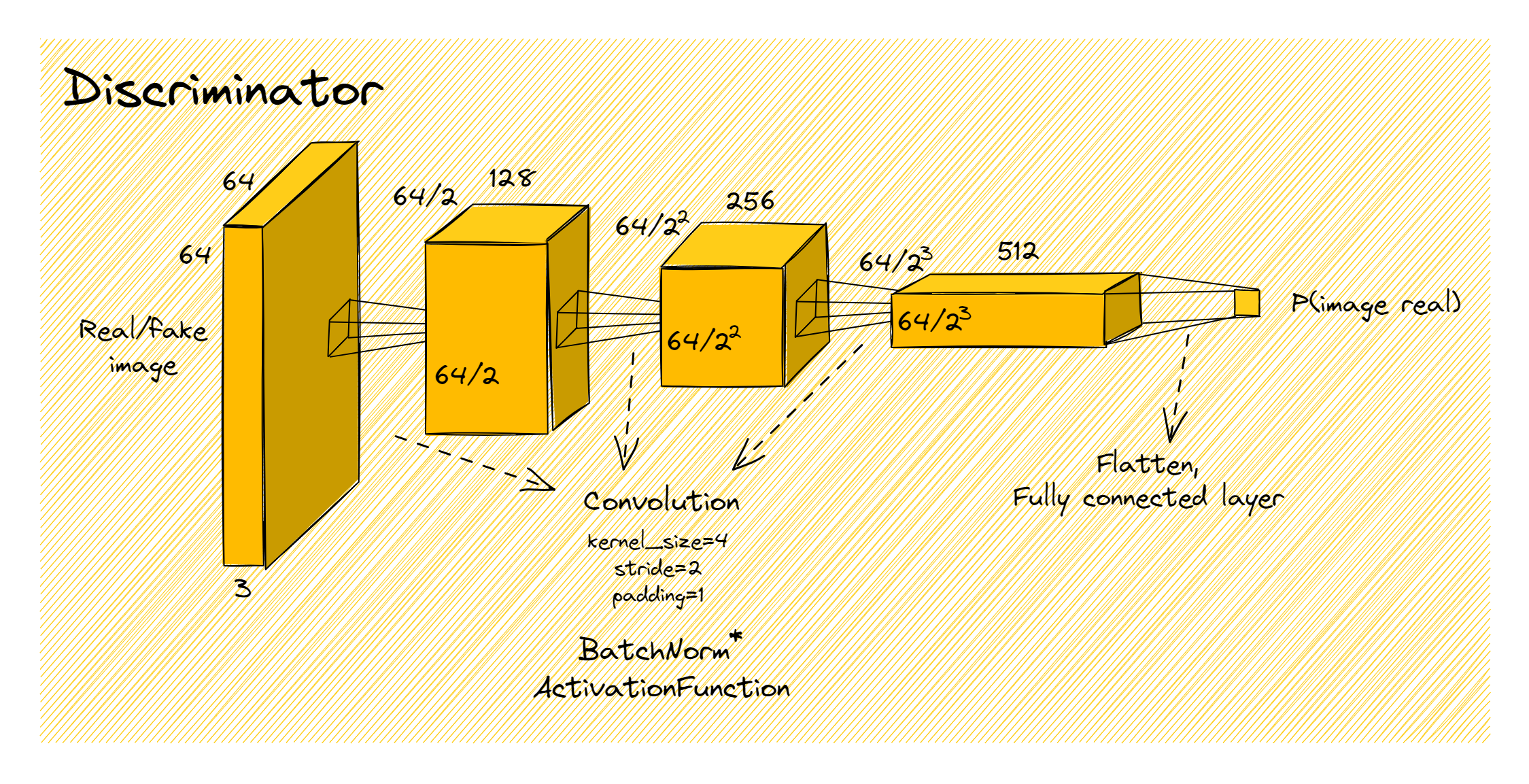
The discriminator starts with a series of blocks of the form (Conv -> BatchNorm -> ActivationFunction). Following the paper's conventions:
- Each convolution should have kernel size 4, stride 2, padding 1.
-
This will (exercise to the reader!) halve the width and height of the image at each step. The number of output channels of each convolution is given by the
hidden_channelsargument. For instance, ifimg_channels=3(because the image is RGB) andhidden_channels=[128, 256, 512], then there will be three convolutions:- the first mapping from
3 -> 128channels, - the second from
128 -> 256, and - the third from
256 -> 512.
- the first mapping from
-
All blocks have a batchnorm layer, except for the very first one.
- All blocks' activation functions are
LeakyReLU.
Lastly, we flatten the output of the final convolutional block, and use a
fully connected layer to map it to a single value
(i.e. a vector of length batch_size). This value is a logit - the
discriminator's pre-sigmoid score for "is this image real?". We deliberately
do not apply a sigmoid here; we convert the logit to a probability
inside the loss, in a numerically stable way (see the
numerical-stability section below). Again, we recommend the Rearrange
module from the einops library for this.
Why pre-sigmoid, and not pre-softmax?
There are only two classes, fake and real, so we can actually get away with just one logit $l$ and then sigmoid it. Why?
Suppose instead we had two output logits $[x,y]$ for each class, and then we softmax in the standard way to get probabilities $[p,1-p]$.
Then $p = \dfrac{\exp(x)}{\exp(x) + \exp(y)}$. Defining $l = x - y$, and letting $\sigma(z) = \dfrac{1}{1 + \exp(-z)}$ be the sigmoid function, we have
None of the convolutions or linear layers in either the discriminator or the generator should have biases.
The diagram below shows what we'd get with the following arguments:
img_size = 64
img_channels = 3
hidden_channels = [128, 256, 512]
Generator
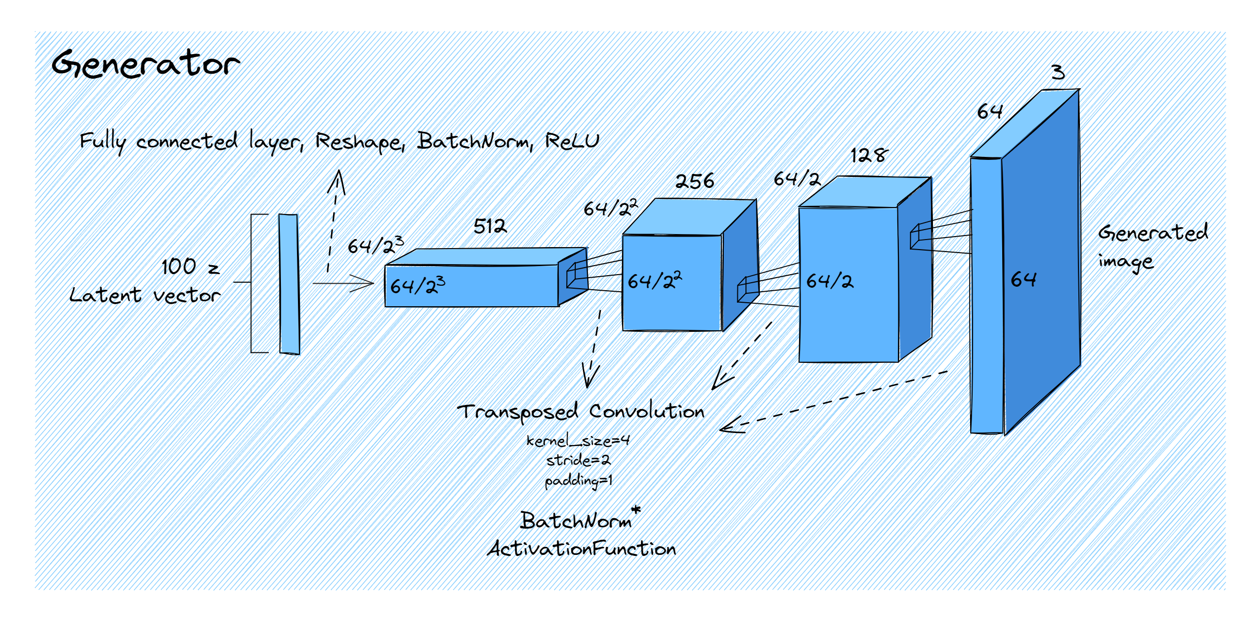
The generator is essentially the mirror image of the discriminator: where the discriminator has convolutions which halve the image size on each layer, the generator has transposed convolutions which double the size on each layer (so apart from the very start of the generator / end of the discriminator, all the activations have the same shape, just in reverse).
We start with the latent vector $\mathbf{z}$ of shape
(batch_size, latent_dim_size), and apply a linear layer and
reshape to get our first tensor which has shape
(batch_size, channels, height, width). The parameters channels and height
(which is equal to width) can be calculated from the img_size and
hidden_channels arguments (remember that image size doubles at each
transposed convolution, and after applying all the transposed
convolutions we'll eventually get back to img_size).
Then, we apply batchnorm and ReLU (not LeakyReLU -
the DCGAN paper prescribes plain ReLU throughout the generator
and LeakyReLU only in the discriminator, so watch out for this asymmetry).
After this, we apply a series of blocks of the form
(ConvTranspose -> BatchNorm -> ActivationFunction).
Following the paper's conventions:
- Each transposed convolution has kernel size 4, stride 2, padding 1.
As for the discriminator, the input and output channels of the transposed
convolutions are determined by the
hidden_channelsargument (although this time from the generator's perspective they're in reverse order). - All blocks have a batchnorm layer, except for the very last one.
- All blocks' activation functions are
ReLU, except for the last one which isTanh.
The diagram below shows what we'd get with the following arguments:
img_size = 64
img_channels = 3
hidden_channels = [128, 256, 512]
latent_dim_size = 100
Exercise - building your GAN
You should implement your code below. We've provided one possible design choice and the corresponding forward functions:
- The generator is made of an initial
project_and_reshapeblock that performs the first linear map, and thenhidden_layerswhich are a stack of blocks each consisting of a (transposed convolution, (optional) batchnorm, activation function). - The discriminator is made of
hidden_layerswhich are a stack of (convolution, optional batchnorm, activation fn) blocks, and a finalclassifierblock which flattens and maps to a single output: the logit (the pre-sigmoid score that the image is real).
We've also given you the DCGAN class: note that we've not included a
forward method here, because you'll usually be calling the forward methods
of the discriminator and generator directly. You can think of the DCGAN class
as essentially a wrapper for both.
If you're stuck, you can import the generator and discriminator from the solutions, and compare it with yours. We've given you this option in place of test functions.
from part2_cnns.utils import print_param_count
from part52_gans import solutions

print_param_count(Generator(), solutions.DCGAN().netG)
print_param_count(Discriminator(), solutions.DCGAN().netD)
Lastly, recall that torchinfo is a useful library for inspecting the architecture of your model. Since it works by running input through your model, it provides another useful way to check your model's architecture is correct (since errors like the wrong convolution size will often cause forward passes to fail).
model = DCGAN().to(device)
x = t.randn(3, 100).to(device)
print(torchinfo.summary(model.netG, input_data=x), end="\n\n")
print(torchinfo.summary(model.netD, input_data=model.netG(x)))
You can also check that the output of your model is the correct shape. Note - we're using a 3-layer model rather than the 4-layer model shown in the diagram and described in the paper.
class Generator(nn.Module):
    def __init__(
        self,
        latent_dim_size: int = 100,
        img_size: int = 64,
        img_channels: int = 3,
        hidden_channels: list[int] = [128, 256, 512],
    ):
        """
        Implements the generator architecture from the DCGAN paper (the diagram at the top
        of page 4). We assume the size of the activations doubles at each layer (so image
        size has to be divisible by 2 ** len(hidden_channels)).

        Args:
            latent_dim_size:
                the size of the latent dimension, i.e. the input to the generator
            img_size:
                the size of the image, i.e. the output of the generator
            img_channels:
                the number of channels in the image (3 for RGB, 1 for grayscale)
            hidden_channels:
                the number of channels in the hidden layers of the generator (starting closest
                to the image and going inward, i.e. in reverse-chronological order for the
                generator, which is why we reverse this list below)
        """
        n_layers = len(hidden_channels)
        assert img_size % (2**n_layers) == 0, (
            "activation size must double at each layer"
        )

        super().__init__()
        # Reverse hidden channels, so they're in chronological order
        hidden_channels = hidden_channels[::-1]
        self.latent_dim_size = latent_dim_size
        self.img_size = img_size
        self.img_channels = img_channels
        self.hidden_channels = hidden_channels

        # Define the first layer, i.e. latent dim -> (512, 8, 8) and reshape
        first_height = img_size // (2**n_layers)
        first_size = hidden_channels[0] * (first_height**2)
        # self.project_and_reshape = ...
        # self.hidden_layers = ...

    def forward(
        self, x: Float[Tensor, "batch latent"]
    ) -> Float[Tensor, "batch channels height width"]:
        x = self.project_and_reshape(x)
        x = self.hidden_layers(x)
        return x


class Discriminator(nn.Module):
    def __init__(
        self,
        img_size: int = 64,
        img_channels: int = 3,
        hidden_channels: list[int] = [128, 256, 512],
    ):
        """
        Implements the discriminator architecture from the DCGAN paper (the mirror image of
        the diagram at the top of page 4). We assume the size of the activations halves at
        each layer (so image size has to be divisible by 2 ** len(hidden_channels)).

        Args:
            img_size:
                the size of the image, i.e. the input of the discriminator
            img_channels:
                the number of channels in the image (3 for RGB, 1 for grayscale)
            hidden_channels:
                the number of channels in the hidden layers of the discriminator (starting
                closest to the image and going inward, i.e. in chronological order for the
                discriminator)
        """
        n_layers = len(hidden_channels)
        assert img_size % (2**n_layers) == 0, "activation size must halve at each layer"

        super().__init__()
        self.img_size = img_size
        self.img_channels = img_channels
        self.hidden_channels = hidden_channels
        self.hidden_layers = ...
        self.classifier = ...

    def forward(
        self, x: Float[Tensor, "batch channels height width"]
    ) -> Float[Tensor, "batch"]:
        x = self.hidden_layers(x)
        x = self.classifier(x)
        return x.squeeze(-1)  # remove dummy `out_channels` dimension


class DCGAN(nn.Module):
    netD: Discriminator
    netG: Generator

    def __init__(
        self,
        latent_dim_size: int = 100,
        img_size: int = 64,
        img_channels: int = 3,
        hidden_channels: list[int] = [128, 256, 512],
    ):
        super().__init__()
        self.latent_dim_size = latent_dim_size
        self.img_size = img_size
        self.img_channels = img_channels
        self.hidden_channels = hidden_channels
        self.netD = Discriminator(img_size, img_channels, hidden_channels)
        self.netG = Generator(latent_dim_size, img_size, img_channels, hidden_channels)
Solution
class Generator(nn.Module):
    def __init__(
        self,
        latent_dim_size: int = 100,
        img_size: int = 64,
        img_channels: int = 3,
        hidden_channels: list[int] = [128, 256, 512],
    ):
        """
        Implements the generator architecture from the DCGAN paper (the diagram at the top
        of page 4). We assume the size of the activations doubles at each layer (so image
        size has to be divisible by 2 ** len(hidden_channels)).

        Args:
            latent_dim_size:
                the size of the latent dimension, i.e. the input to the generator
            img_size:
                the size of the image, i.e. the output of the generator
            img_channels:
                the number of channels in the image (3 for RGB, 1 for grayscale)
            hidden_channels:
                the number of channels in the hidden layers of the generator (starting closest
                to the image and going inward, i.e. in reverse-chronological order for the
                generator, which is why we reverse this list below)
        """
        n_layers = len(hidden_channels)
        assert img_size % (2**n_layers) == 0, (
            "activation size must double at each layer"
        )

        super().__init__()
        # Reverse hidden channels, so they're in chronological order
        hidden_channels = hidden_channels[::-1]
        self.latent_dim_size = latent_dim_size
        self.img_size = img_size
        self.img_channels = img_channels
        self.hidden_channels = hidden_channels

        # Define the first layer, i.e. latent dim -> (512, 8, 8) and reshape
        first_height = img_size // (2**n_layers)
        first_size = hidden_channels[0] * (first_height**2)

        self.project_and_reshape = Sequential(
            Linear(latent_dim_size, first_size, bias=False),
            Rearrange("b (ic h w) -> b ic h w", h=first_height, w=first_height),
            nn.BatchNorm2d(hidden_channels[0]),
            ReLU(),
        )

        # Equivalent, but using conv rather than linear:
        # self.project_and_reshape = Sequential(
        #     Rearrange("b ic -> b ic 1 1"),
        #     nn.ConvTranspose2d(latent_dim_size, hidden_channels[0], first_height, 1, 0, bias=False),
        #     nn.BatchNorm2d(hidden_channels[0]),
        #     ReLU(),
        # )

        # Get list of input & output channels for the convolutional blocks
        in_channels = hidden_channels
        out_channels = hidden_channels[1:] + [img_channels]

        # Define all the convolutional blocks (conv_transposed -> batchnorm -> activation)
        conv_layer_list = []
        for i, (c_in, c_out) in enumerate(zip(in_channels, out_channels)):
            conv_layer = [
                nn.ConvTranspose2d(c_in, c_out, 4, 2, 1, bias=False),
                ReLU() if i < n_layers - 1 else Tanh(),
            ]
            if i < n_layers - 1:
                conv_layer.insert(1, nn.BatchNorm2d(c_out))
            conv_layer_list.append(Sequential(*conv_layer))

        self.hidden_layers = Sequential(*conv_layer_list)

    def forward(
        self, x: Float[Tensor, "batch latent"]
    ) -> Float[Tensor, "batch channels height width"]:
        x = self.project_and_reshape(x)
        x = self.hidden_layers(x)
        return x


class Discriminator(nn.Module):
    def __init__(
        self,
        img_size: int = 64,
        img_channels: int = 3,
        hidden_channels: list[int] = [128, 256, 512],
    ):
        """
        Implements the discriminator architecture from the DCGAN paper (the mirror image of
        the diagram at the top of page 4). We assume the size of the activations halves at
        each layer (so image size has to be divisible by 2 ** len(hidden_channels)).

        Args:
            img_size:
                the size of the image, i.e. the input of the discriminator
            img_channels:
                the number of channels in the image (3 for RGB, 1 for grayscale)
            hidden_channels:
                the number of channels in the hidden layers of the discriminator (starting
                closest to the image and going inward, i.e. in chronological order for the
                discriminator)
        """
        n_layers = len(hidden_channels)
        assert img_size % (2**n_layers) == 0, "activation size must halve at each layer"

        super().__init__()
        self.img_size = img_size
        self.img_channels = img_channels
        self.hidden_channels = hidden_channels

        # Get list of input & output channels for the convolutional blocks
        in_channels = [img_channels] + hidden_channels[:-1]
        out_channels = hidden_channels

        # Define all the convolutional blocks (conv -> batchnorm -> activation)
        conv_layer_list = []
        for i, (c_in, c_out) in enumerate(zip(in_channels, out_channels)):
            conv_layer = [
                Conv2d(c_in, c_out, 4, 2, 1),
                LeakyReLU(0.2),
            ]
            if i > 0:
                conv_layer.insert(1, nn.BatchNorm2d(c_out))
            conv_layer_list.append(Sequential(*conv_layer))

        self.hidden_layers = Sequential(*conv_layer_list)

        # Define the last layer, i.e. reshape and (512, 8, 8) -> real/fake classification
        final_height = img_size // (2**n_layers)
        final_size = hidden_channels[-1] * (final_height**2)
        self.classifier = Sequential(
            Rearrange("b c h w -> b (c h w)"),
            Linear(final_size, 1, bias=False),
        )
        # Equivalent, but using conv rather than linear:
        # self.classifier = Sequential(
        #     Conv2d(out_channels[-1], 1, final_height, 1, 0),
        #     Rearrange("b c h w -> b (c h w)"),
        # )

    def forward(
        self, x: Float[Tensor, "batch channels height width"]
    ) -> Float[Tensor, "batch"]:
        x = self.hidden_layers(x)
        x = self.classifier(x)
        return x.squeeze(-1)  # remove dummy `out_channels` dimension
Exercise - Weight initialisation
The paper mentions at the end of page 3 that all weights were initialized from a $N(\mu = 0, \sigma^2 = 0.02^2)$ distribution, i.e. zero-centered with standard deviation 0.02. This applies to the convolutional and convolutional transpose layers' weights (plus the weights in the linear classifier), but the BatchNorm layers' weights should be initialised from $N(1, 0.02^2)$ (since 1 is their default value). The BatchNorm biases should all be set to zero.
You can fill in the following function to initialise your weights, and call it within the __init__ method of your DCGAN. (Hint: you can use the functions
nn.init.normal_
and nn.init.constant_ here.)
def initialize_weights(model: nn.Module) -> None:
    """
    Initializes weights according to the DCGAN paper (details at the end of page 3 of the DCGAN
    paper), by modifying the weights of the model in place.
    """
    raise NotImplementedError()


tests.test_initialize_weights(initialize_weights, nn.ConvTranspose2d, Conv2d, Linear, nn.BatchNorm2d)
Solution
def initialize_weights(model: nn.Module) -> None:
    """
    Initializes weights according to the DCGAN paper (details at the end of page 3 of the DCGAN
    paper), by modifying the weights of the model in place.
    """
    for module in model.modules():
        # Match torch's `nn.ConvTranspose2d` (used by default in the GAN code) AND any class
        # named `ConvTranspose2d` (so the VAEs section's bonus implementation is also picked up
        # if a student swaps it in).
        is_conv_transpose = isinstance(module, nn.ConvTranspose2d) or type(module).__name__ == "ConvTranspose2d"
        if is_conv_transpose or isinstance(module, (Conv2d, Linear)):
            nn.init.normal_(module.weight.data, 0.0, 0.02)
        elif isinstance(module, nn.BatchNorm2d):
            nn.init.normal_(module.weight.data, 1.0, 0.02)
            nn.init.constant_(module.bias.data, 0.0)
Note - the tests for this aren't maximally strict, but don't worry if you don't get things exactly right, since your model will still probably train successfully. If you think you've got the architecture right but your model still isn't training, you might want to return here and check your initialisation.
class DCGAN(nn.Module):
    netD: Discriminator
    netG: Generator

    def __init__(
        self,
        latent_dim_size: int = 100,
        img_size: int = 64,
        img_channels: int = 3,
        hidden_channels: list[int] = [128, 256, 512],
    ):
        super().__init__()
        self.latent_dim_size = latent_dim_size
        self.img_size = img_size
        self.img_channels = img_channels
        self.hidden_channels = hidden_channels
        self.netD = Discriminator(img_size, img_channels, hidden_channels)
        self.netG = Generator(latent_dim_size, img_size, img_channels, hidden_channels)
        initialize_weights(self.netD)
        initialize_weights(self.netG)

model = DCGAN().to(device)
x = t.randn(3, 100).to(device)
print(torchinfo.summary(model.netG, input_data=x), end="\n\n")
print(torchinfo.summary(model.netD, input_data=model.netG(x)))
==========================================================================================
Layer (type:depth-idx)                   Output Shape              Param #
==========================================================================================
Generator                                [3, 3, 64, 64]            --
├─Sequential: 1-1                        [3, 512, 8, 8]            --
│    └─Linear: 2-1                       [3, 32768]                3,276,800
│    └─Rearrange: 2-2                    [3, 512, 8, 8]            --
│    └─BatchNorm2d: 2-3                  [3, 512, 8, 8]            1,024
│    └─ReLU: 2-4                         [3, 512, 8, 8]            --
├─Sequential: 1-2                        [3, 3, 64, 64]            --
│    └─Sequential: 2-5                   [3, 256, 16, 16]          --
│    │    └─ConvTranspose2d: 3-1         [3, 256, 16, 16]          2,097,152
│    │    └─BatchNorm2d: 3-2             [3, 256, 16, 16]          512
│    │    └─ReLU: 3-3                    [3, 256, 16, 16]          --
│    └─Sequential: 2-6                   [3, 128, 32, 32]          --
│    │    └─ConvTranspose2d: 3-4         [3, 128, 32, 32]          524,288
│    │    └─BatchNorm2d: 3-5             [3, 128, 32, 32]          256
│    │    └─ReLU: 3-6                    [3, 128, 32, 32]          --
│    └─Sequential: 2-7                   [3, 3, 64, 64]            --
│    │    └─ConvTranspose2d: 3-7         [3, 3, 64, 64]            6,144
│    │    └─Tanh: 3-8                    [3, 3, 64, 64]            --
==========================================================================================
Total params: 5,906,176
Trainable params: 5,906,176
Non-trainable params: 0
Total mult-adds (Units.GIGABYTES): 3.31
==========================================================================================
Input size (MB): 0.00
Forward/backward pass size (MB): 11.30
Params size (MB): 23.62
Estimated Total Size (MB): 34.93
==========================================================================================

==========================================================================================
Layer (type:depth-idx)                   Output Shape              Param #
==========================================================================================
Discriminator                            [3]                       --
├─Sequential: 1-1                        [3, 512, 8, 8]            --
│    └─Sequential: 2-1                   [3, 128, 32, 32]          --
│    │    └─Conv2d: 3-1                  [3, 128, 32, 32]          6,144
│    │    └─LeakyReLU: 3-2               [3, 128, 32, 32]          --
│    └─Sequential: 2-2                   [3, 256, 16, 16]          --
│    │    └─Conv2d: 3-3                  [3, 256, 16, 16]          524,288
│    │    └─BatchNorm2d: 3-4             [3, 256, 16, 16]          512
│    │    └─LeakyReLU: 3-5               [3, 256, 16, 16]          --
│    └─Sequential: 2-3                   [3, 512, 8, 8]            --
│    │    └─Conv2d: 3-6                  [3, 512, 8, 8]            2,097,152
│    │    └─BatchNorm2d: 3-7             [3, 512, 8, 8]            1,024
│    │    └─LeakyReLU: 3-8               [3, 512, 8, 8]            --
├─Sequential: 1-2                        [3, 1]                    --
│    └─Rearrange: 2-4                    [3, 32768]                --
│    └─Linear: 2-5                       [3, 1]                    32,768
==========================================================================================
Total params: 2,661,888
Trainable params: 2,661,888
Non-trainable params: 0
Total mult-adds (Units.MEGABYTES): 824.28
==========================================================================================
Input size (MB): 0.15
Forward/backward pass size (MB): 7.86
Params size (MB): 10.65
Estimated Total Size (MB): 18.66
==========================================================================================
Training loop
Recall, the goal of training the discriminator is to maximize the probability of correctly classifying a given input as real or fake. The goal of the generator is to produce images to fool the discriminator. This is framed as a minimax game, where the discriminator and generator try to solve the following:
The literature on minimax games is extensive, so we won't go into it here. It's better to understand this formula on an intuitive level:
- Given a fixed $G$ (generator), the goal of the discriminator is to produce high values for $D$ when fed real images $x$, and low values when fed fake images $G(\mathbf{z})$.
- The generator $G$ is searching for a strategy where, even if the discriminator $D$ was optimal, it would still find it hard to distinguish between real and fake images with high confidence.
Since we can't know the true distribution of $x$ (one can imagine the platonic distribution where images are drawn from) we instead estimate the expression above by calculating it over a batch of real images $x$ (and some random noise $\mathbf{z}$). This gives us a loss function to train against (since $D$ wants to maximise this value, and $G$ wants to minimise this value). For each batch, we perform gradient descent on the discriminator and then on the generator.
Training the discriminator
We take the following steps:
- Zero the gradients of $D$.
- This is important because if the last thing we did was evaluate $D(G(\mathbf{z}))$ (in order to update the parameters of $G$), then $D$ will have stored gradients from that backward pass.
- Generate random noise $\mathbf{z}$, and compute $D(G(\mathbf{z}))$.
Compute the empirical mean of $\log(1 - D(G(\mathbf{z})))$ over the batch dimension,
and we have the first part of our loss function.
- Note - you can use the same random noise (and even the same fake image) as in the generator step. But make sure you're using the detached version, because we don't want gradients to propagate back through the generator!
- Take the real images $x$ in the current batch, and use that to compute $\log(D(x))$. This gives us the second part of our loss function.
- We now add the two terms together. The discriminator wants to maximise this expression, so as usual we flip its sign and minimise the result with gradient descent.
Tip - when calculating $D(G(z))$, for the purpose of training the discriminator, it's best to first calculate $G(z)$ then call detach on this tensor before passing it to $D$. This is because you then don't need to worry about gradients accumulating for $G$.
Training the generator
We take the following steps:
- Zero the gradients of $G$.
- Generate random noise $\mathbf{z}$, and compute $D(G(\mathbf{z}))$.
- We don't use $\log(1 - D(G(\mathbf{z})))$ to calculate our loss function, instead we use $\log(D(G(\mathbf{z})))$ (which the generator wants to maximise, so again we minimise its negative).
Question - can you explain why we use $\log(D(G(\mathbf{z})))$? (The Google reading material mentions this but doesn't really explain it.)
Answer
Early in learning, when the generator is really bad at producing realistic images, it will be easy for the discriminator to distinguish between them. So $\log(1 - D(G(\mathbf{z})))$ will be very close to $\log(1) = 0$. The gradient of $\log$ at this point is quite flat, so there won't be a strong gradient with which to train $G$. To put it another way, a marginal improvement in $G$ will have very little effect on the loss function. On the other hand, $\log(D(G(\mathbf{z})))$ tends to negative infinity as $D(G(\mathbf{z}))$ gets very small. So the gradients here are very steep, and a small improvement in $G$ goes a long way.
It's worth emphasising that these two functions are both monotonic in opposite directions, so maximising one is equivalent to minimising the other. We haven't changed anything fundamental about how the GAN works; this is just a trick to help with gradient descent.
(Optional) A note on numerical stability: working in logit space
This section can be skipped without loss of continuity. If you don't care about details of numerical stability, the TL;DR is "use F.logsigmoid to compute $\log \sigma(z)$", rather than
t.log(F.sigmoid(x))or similar. If you care how and why, read on.
Details of numerically evaluating logsigmoid
Our loss needs $\log D(x)$ and $\log(1 - D(G(z)))$. Since $D(x) = \sigma(l)$ where $l$ is the discriminator's logit, these are really $\log \sigma(z)$ terms. If we compute this the naive way (apply sigmoid, then take its log) this can numerically blow-up.
Here's why. When the discriminator gets confident, its logit $z$ grows large in magnitude and $\sigma(z)$ saturates towards $0$ or $1$ exponentially fast.
Why does $\sigma(z)$ saturate exponentially fast?
$1+\exp(-z) > \exp(-z)$ so $\sigma(z) = \dfrac{1}{1+\exp(-z)} < \exp(-z)^{-1} = \exp(z)$, so $\sigma(z) \to 0$ exponentially fast as $z \to -\inf$. Proving $\sigma(z) \to 1$ exponentially fast as $z \to +\inf$ is a similar exercise.In float arithmetic $\sigma(-100)$ doesn't just get small - it rounds to exactly 0.0,
>>> t.sigmoid(t.Tensor([-100])) == 0
tensor([True])
and then t.log(0.0) $= -\infty$, so the loss becomes inf/nan and the run dies.
The fix is to compute a fused, numerically-stable $\log \sigma(z)$ directly
from the logit, so the underflowing probability is never formed. This is why
our discriminator returns a raw logit (rather than putting the sigmoid inside
the network), and why the loss uses F.logsigmoid:
(the middle one uses $1 - \sigma(z) = \sigma(-z)$).
PyTorch provides F.logsigmoid for this purpose, which is implemented
under the hood as
Every exponent here is $\le 0$, so exp can never overflow,
and log1p never sees log(0).
Derivation of numerically stable log_sigmoid
Start from the definition:
The fix is the log-sum-exp trick (the same one that stabilises softmax): factor the larger of the two exponents out of the sum. The terms inside $1 + e^{-z}$ have exponents $0$ and $-z$, so factor out $e^{m}$ with $m = \max(0, -z)$:
log1p itself applies the same idea one level down to stay accurate for tiny arguments - see PyTorch's kernel.)
This is exactly what PyTorch's F.logsigmoid does under the hood:
see its CUDA kernel, which computes min(x, 0) - log1p(exp(-|x|))
(as well as providing a numerically stable form of the backward method
for backpropagation).
Defined for PyTorch here
which borrows the Numpy implementation which is described in Theorem 4 of this paper. Okay, what about
log1p? def log1p_theorem4(z):
z = complex(z)
u = z + 1
if u == 1:
return z
elif u - 1 == z:
return np.log(u)
else:
return np.log(u)*(z/(u - 1))
x+1 == 1 would evaluate to true
when x is so small that x+1 gets rounded off to 1.)
There's a reason numerical analysis is an entire discipline of study!
Was that all necessary?
Yes! Without it, our GAN implementation regularly NaNs out!
This training code used to sometimes fail and throw NaNs midway
through training until it was addressed. I invite you to replace
F.logsigmoid(...) with t.log(F.sigmoid(...)) and you can see for yourself
what happens.
Optimizers
The generator and discriminator will have separate optimizers (this makes
sense, since we'll have separate training steps for these two, and
both are "trying" to optimize different things). The
paper describes using an Adam optimizer
with learning rate 0.0002, and momentum parameters
$\beta_1 = 0.5, \beta_2 = 0.999$. This is set up for you already,
in the __init__ block below.
The discriminator and generator each want to maximize a log-likelihood, so
their losses lossD/lossG are the negative log-likelihoods, which we
minimize as usual with loss.backward() followed by optimizer.step().
Why does the discriminator get a higher learning rate than the generator?
Most GAN advice you'll read says the opposite: throttle the discriminator, so it doesn't overpower the generator and leave it with no useful gradient to learn from. The TTUR paper is the usual citation.
At least for our architecture, a hyperparameter sweep revealed the opposite story:
Measured on CelebA, FID against 10k real images (lower is better), batch 64, equal wall-clock:
lr_D |
lr_G |
FID |
|---|---|---|
| 2e-4 | 4e-4 | 63.5 |
| 4e-4 | 4e-4 | 43.4 |
| 8e-4 | 2e-4 | 23.9 |
| 1.6e-3 | 4e-4 | 22.1 |
| 3.2e-3 | 8e-4 | 31.9 (starts to destabilise) |
Gradient Clipping
Gradient clipping is a useful technique for improving the stability of
certain training loops, especially those like DCGANs which have potentially
unstable loss functions. The idea is that you clip the gradients of your
weights to some fixed threshold during backprop, and use these clipped
gradients to update the weights. This can be done using
nn.utils.clip_grad_norm, which is called between the
loss.backward() and optimizer.step() methods (since it directly modifies
the .grad attributes of your weights). You shouldn't find this absolutely
necessary to train your models, however it might help to clip the gradients
to a value like 1.0 for your generator & discriminator. We've given you
this as an optional parameter to use in your DCGANArgs dataclass.
Exercise - implement GAN training loop
You should now implement your training loop below. We've filled in the
__init__ method for you, as well as log_samples method which determines
the core structure of the training loop. Your task is to:
-
Fill in the two functions
training_step_discriminatorandtraining_step_generator, which perform a single gradient step on the discriminator and generator respectively.-
Note that the discriminator training function takes two arguments: the real and fake image (in the notation above, $x$ and $G(\mathbf{z})$), because it trains to distinguish real and fake. The generator training function only takes the fake image $\mathbf{z}$, because it trains to fool the discriminator (there's nothing the generator could possibly do that would affect how the discriminator feels about real images). It matters that these are two separate calls to
netDrather than one batched call - see the dropdown at the end of this section for what happens if you batch them. -
Also note, you should increment
self.steponly once per (discriminator & generator) step, not for both. - Fill in the
trainmethod, which should perform the training loop over the number of epochs specified inargs.epochs. This will be similar to previous training loops, but with a few key differences we'll highlight here: - You'll need to compute both losses from
training_step_generatorandtraining_step_discriminator. For the former you should pass in just the fake image (you're only training the generator to produce better fake images), for the latter you should pass in the real image and the detached fake image i.e.img_fake.detach()(because you're training the discriminator to tell real from fake, and you don't want gradients propagating back to the generator).- The fake image should be created from random noise
$\mathbf{z}$ =
t.randn(batch_size, latent_dim_size)and passing it into your generator.
- The fake image should be created from random noise
$\mathbf{z}$ =
- Once again the trainloader gives us an iterable of
(img, label)but we don't need to use the labels (because all these images are real, and that's all we care about).
-
-
Don't forget to transform the images once they're on the GPU, and before you feed them to the discriminator, with
img_real = self.trainset.transform(img_real.to(device)). The dataset hands you rawuint8images; this is what scales them to floats, normalizes them, and (for CelebA) crops them down to 64x64. - Don't forget to compute the objective terms in a numerically stable way using
F.logsigmoidas described earlier:
(the middle term uses $1 - \sigma(z) = \sigma(-z)$).
The loss to minimize for the discriminator is
Again, we recommend not using wandb until you've got your non-wandb based
code working without errors. Once the generator loss is going down
(or at least not exploding!) then you can enable it. However, an important
note - the generator loss going down does not imply the model is working,
and vice-versa! For training systems as unstable as GANs, the best you can do
is often just inspecting the output. Although it varies depending on details
of the hardware and dataset & model you're training with, at least for these
exercises if your generator's output doesn't resemble anything like a face
after the first epoch, then something's probably going wrong in your code.
Consider lossD and lossG (the negative log-likelihoods we minimize for the
discriminator and generator) to not represent something meaningful about the
current performance of the model, but more like an
electrocardiogram (ECG)
of the training run: if one of them flatlines, the "patient" is dead.
Both losses are negative log-probabilities, so they're always $\geq 0$, with $0$ meaning "perfect" (for
that network). The useful reference point is a discriminator that outputs $D = \tfrac12$ for every image,
i.e. one that can't tell real from fake at all:What values of
lossD and lossG should I expect?
You'll see values close to these at the very start of training (the $N(0, 0.02^2)$ weight initialisation
makes every logit $\approx 0$, and $\sigma(0) = \tfrac12$), and they're also where an ideal run would end
up, with a perfect generator and a discriminator reduced to guessing. In between, lossD sitting below
$\ln 4$ means the discriminator is beating chance. If lossD heads towards $0$ while lossG climbs, the
discriminator is winning outright, and the generator is about to stop getting a useful training signal.
Where does ln 4 really come from? (optional, uses the Jensen-Shannon divergence)
The **Jensen-Shannon divergence** between the real distribution $P$ and the generated distribution $Q$ is the average KL divergence from each of them to their 50/50 mixture $M = \tfrac12(P + Q)$:Why two separate calls to netD? Couldn't we batch them together?
Disclaimer: Discovered and written by Claude.
It looks like you could: netD(t.cat([img_real, img_fake])) computes the same logits in one
call instead of two, which on this model is measurably faster (about 1.24x, because the
discriminator's many small operations are the bottleneck).
It also completely destroys training. We measured it: FID goes from 22 to 388, which is worse than feeding the metric pure random noise, and the generator never improves at all from the very first evaluation.
The culprit is BatchNorm. Inside the discriminator, batch normalization computes its mean
and variance over the whole batch - so if that batch contains real images in one half and
fake images in the other, each image's output starts to depend on the other images it
happens to be batched with. The discriminator can then separate the two halves using
batch-level statistics rather than by looking at any individual image, which is a free and
perfect answer. It stops learning anything about what makes an image realistic, the
generator's gradient stops carrying that information too, and training never gets going.
This is a very hard to find gotcha, as BatchNorm (unlike most other PyTorch operations, and even unlike other normalizations like LayerNorm) has cross-batch dependencies during training. Since real and fake images are drawn from different distributions (at least while the generator is bad), we want to normalize them independently, or it is too easy for the discriminator to latch onto this as a signal.
Also, unlike in [0.2] and [0.3] where we normalized the images
to have zero mean and unit variance, here, we just rescale the pixels
such that they are always in the range [-1,1]. This has been done
for you with TANH_RANGE_TRANSFORM.
Why use the Tanh normalization over zero-mean/unit-std?
The generator ends in Tanh, so any image it produces must be in the range [-1, 1] too. MNIST's default transform normalizes by its mean/std (for the VAEs section), giving [-0.42, 2.82], a range the generator can't reach, so the discriminator would win trivially by just looking at the brightness of the maximum pixel. Hence we ask for the [-1, 1] transform explicitly, whichever dataset this is.
@dataclass
class DCGANArgs:
    """
    Class for the arguments to the DCGAN (training and architecture).
    Note, we use field(default_factory=...) when our default value is a mutable object.
    """

    # architecture
    latent_dim_size: int = 100
    hidden_channels: list[int] = field(default_factory=lambda: [128, 256, 512])

    # data & training
    dataset: Literal["MNIST", "CELEB"] = "CELEB"
    batch_size: int = 64
    epochs: int = 3
    lr: float = 0.0002
    lr_G: float | None = None  # generator LR (TTUR); falls back to `lr` if None
    lr_D: float | None = None  # discriminator LR (TTUR); falls back to `lr` if None
    betas: tuple[float, float] = (0.5, 0.999)
    clip_grad_norm: float | None = 1.0

    # performance
    compile: bool = False  # optional ~2x speed-up, off by default

    # logging
    use_wandb: bool = False
    wandb_project: str | None = "day5-gan"
    wandb_name: str | None = None
    log_every_n_steps: int = 250

    def __post_init__(self):
        # Two Time-Scale Update Rule (TTUR): allow separate generator/discriminator learning
        # rates. Both default to the shared `lr` unless explicitly overridden.
        if self.lr_G is None:
            self.lr_G = self.lr
        if self.lr_D is None:
            self.lr_D = self.lr


class DCGANTrainer:
    def __init__(self, args: DCGANArgs):
        self.args = args

        self.trainset = get_dataset(self.args.dataset, transform=TANH_RANGE_TRANSFORM)
        # `drop_last=True` keeps every batch the same shape, which matters when we compile below
        self.trainloader = DataLoader(
            self.trainset, batch_size=args.batch_size, shuffle=True, num_workers=NUM_WORKERS, drop_last=True
        )

        img_batch = self.trainset.transform(next(iter(self.trainloader))[0])
        batch, img_channels, img_height, img_width = img_batch.shape
        assert img_height == img_width

        self.model = DCGAN(args.latent_dim_size, img_height, img_channels, args.hidden_channels).to(device).train()

        if args.compile and device.type == "cuda":
            self.model.netG = t.compile(self.model.netG)
            self.model.netD = t.compile(self.model.netD)

        self.optG = t.optim.Adam(self.model.netG.parameters(), lr=args.lr_G, betas=args.betas)
        self.optD = t.optim.Adam(self.model.netD.parameters(), lr=args.lr_D, betas=args.betas)

        # The *same* noise every time we log samples, so successive plots show a single set of faces
        # improving rather than a fresh random set each time.
        self.fixed_noise = t.randn(10, args.latent_dim_size, device=device)

    def training_step_discriminator(
        self,
        img_real: Float[Tensor, "batch channels height width"],
        img_fake: Float[Tensor, "batch channels height width"],
    ) -> Float[Tensor, ""]:
        """
        Generates a real and fake image, and performs a gradient step on the discriminator to
        minimize -(log(D(x)) + log(1-D(G(z)))). Logs to wandb if enabled.
        """
        raise NotImplementedError()

    def training_step_generator(
        self, img_fake: Float[Tensor, "batch channels height width"]
    ) -> Float[Tensor, ""]:
        """
        Performs a gradient step on the generator to minimize -log(D(G(z))). Logs to wandb if enabled.
        """
        raise NotImplementedError()

    @t.inference_mode()
    def log_samples(self) -> None:
        """
        Performs evaluation by passing the 10 fixed noise vectors in `self.fixed_noise` through the
        generator, then optionally logging the results to Weights & Biases.
        """
        assert self.step > 0, "First call should come after a training step. Remember to increment `self.step`."
        self.model.netG.eval()

        output = self.model.netG(self.fixed_noise)
        # Clip values to make the visualization clearer
        output = output.clamp(output.quantile(0.01), output.quantile(0.99))
        # Log to weights and biases
        if self.args.use_wandb:
            output = einops.rearrange(output, "b c h w -> b h w c").cpu().numpy()
            wandb.log({"images": [wandb.Image(arr) for arr in output]}, step=self.step)
        else:
            self.live_image.update(output)

        self.model.netG.train()

    def train(self) -> DCGAN:
        """Performs a full training run."""
        self.step = 0
        self.live_image = LiveImage()  # `log_samples` overwrites this in place
        if self.args.use_wandb:
            wandb.init(project=self.args.wandb_project, name=self.args.wandb_name)

        # One progress bar for the whole run (rather than a new one each epoch)
        progress_bar = tqdm(total=self.args.epochs * len(self.trainloader), ascii=True)

        for epoch in range(self.args.epochs):
            for img_real, label in self.trainloader:
                # YOUR CODE HERE - fill in the training step for generator & discriminator

        progress_bar.close()
        if self.args.use_wandb:
            wandb.finish()

        return self.model
Help - I'm getting OOMs/crashes when I try to use the trainloader
This is a known issue on MacOS machines. To fix this, try adding multiprocessing_context="fork" to your DataLoader instantiation.
Solution
def training_step_discriminator(
    self,
    img_real: Float[Tensor, "batch channels height width"],
    img_fake: Float[Tensor, "batch channels height width"],
) -> Float[Tensor, ""]:
    """
    Generates a real and fake image, and performs a gradient step on the discriminator to minimize
    -(log(D(x)) + log(1-D(G(z)))). Logs to wandb if enabled.
    """
    # Zero gradients
    self.optD.zero_grad()

    logits_real = self.model.netD(img_real)
    logits_fake = self.model.netD(img_fake)

    lossD = -(F.logsigmoid(logits_real).mean() + F.logsigmoid(-logits_fake).mean())

    lossD.backward()
    if self.args.clip_grad_norm is not None:
        nn.utils.clip_grad_norm_(self.model.netD.parameters(), self.args.clip_grad_norm)
    self.optD.step()

    if self.args.use_wandb:
        wandb.log(dict(lossD=lossD), step=self.step)
    return lossD


def training_step_generator(self, img_fake: Float[Tensor, "batch channels height width"]) -> Float[Tensor, ""]:
    """
    Performs a gradient step on the generator to minimize -log(D(G(z))). Logs to wandb if enabled.
    """
    # Zero gradients
    self.optG.zero_grad()

    logits_fake = self.model.netD(img_fake)

    lossG = -F.logsigmoid(logits_fake).mean()
    lossG.backward()
    if self.args.clip_grad_norm is not None:
        nn.utils.clip_grad_norm_(self.model.netG.parameters(), self.args.clip_grad_norm)
    self.optG.step()

    if self.args.use_wandb:
        wandb.log(dict(lossG=lossG), step=self.step)
    return lossG


def train(self) -> DCGAN:
    """Performs a full training run."""
    self.step = 0
    if self.args.use_wandb:
        wandb.init(project=self.args.wandb_project, name=self.args.wandb_name)

    # One progress bar for the whole run (rather than a new one each epoch)
    progress_bar = tqdm(total=self.args.epochs * len(self.trainloader), ascii=True)

    for epoch in range(self.args.epochs):
        for img_real, label in self.trainloader:
            # Generate random noise & fake image
            img_real = self.trainset.transform(img_real.to(device))
            noise = t.randn(img_real.shape[0],
                            self.args.latent_dim_size,
                            device=device)
            img_fake = self.model.netG(noise)

            # Training steps
            lossD = self.training_step_discriminator(img_real, img_fake.detach())
            lossG = self.training_step_generator(img_fake)

            # Update progress bar
            self.step += 1
            progress_bar.set_description(
                f"{epoch=}, {lossD=:.4f}, {lossG=:.4f}, batches={self.step}", refresh=False
            )
            progress_bar.update()

            # Log batch of data
            if self.step % self.args.log_every_n_steps == 0:
                self.log_samples()

    progress_bar.close()
    if self.args.use_wandb:
        wandb.finish()

    return self.model
Once you've written your code, here are some default arguments for MNIST and CelebA you can try out.
Note that the MNIST model is very small in comparison to CelebA - if you make it any larger, you fall into a very common GAN failure mode where the discriminator becomes perfect (loss goes to zero) and the generator is unable to get a gradient signal to produce better images - see next section for a discussion of this. Larger architectures are generally more likely to fall into this failure mode, and empirically it seems to happen more for MNIST than for CelebA which is why we generally recommend using the CelebA dataset & architecture for this exercise - although this failure mode can happen in both cases!
# Arguments for CelebA
args = DCGANArgs(
    dataset="CELEB",
    hidden_channels=[128, 256, 512],
    batch_size=64,  # if you get OOM errors, reduce this!
    epochs=5,
    lr_D=8e-4,  # separate LRs for generator and discriminator
    lr_G=2e-4,
    use_wandb=False,
    compile=False, # toggle me once you have the bugs ironed out
)
trainer = DCGANTrainer(args)
dcgan_celeb = trainer.train()
Click to see an example of the output you should be producing by the end of this CelebA training run.
After 250 batches (16k images), the generator has already found the rough layout of a face: a rough oval framed by hair, dark pits for eyes, and a rough nose and mouth. The background still contains a lot of blocky pixel noise. My guess is an artifact from initialization of the convolution filters bleeding through.
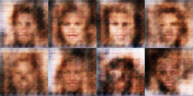
After 2000 batches (128k images), these are recognisably different people, with varied hair colour, lighting and expressions (some are smiling), though the features are still smeared and the backgrounds are blurry gradients.
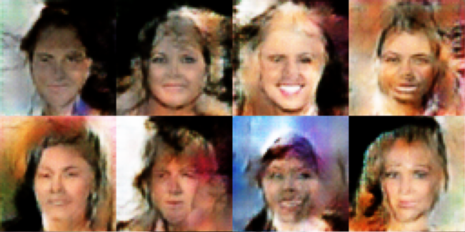
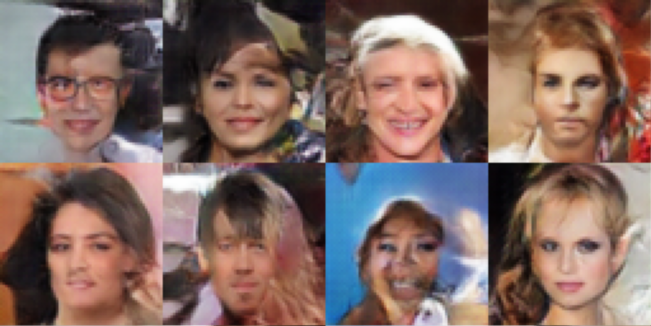
At the end of training (5 epochs, 15,825 batches, approx 1M images), most samples are sharp, varied faces with plausible backgrounds and details like glasses, though some are still heavily warped and distorted. Presumably it's enough to fool the simple discriminator. Longer training, or larger models would probably get a more capable result.
# Arguments for MNIST
args = DCGANArgs(
    dataset="MNIST",
    hidden_channels=[12, 24],
    epochs=20,
    batch_size=128,
    use_wandb=False,
    compile=False, # toggle me once you have the bugs ironed out
)
trainer = DCGANTrainer(args)
dcgan_mnist = trainer.train()
Click to see an example of the output you should be producing by the end of this MNIST training run.
After 250 batches (32k images), the output is still flat grey + noise: the generator hasn't learned anything yet. Don't give up yet! In our run the samples stayed flat grey until roughly 1250 batches (about 2.5 epochs), then faint texture appeared.

After 2000 batches (256k images), there are bright, blobby stroke shapes on a noisy dark-grey background. They're roughly digit-sized and digit-shaped.
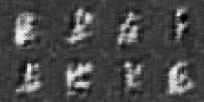
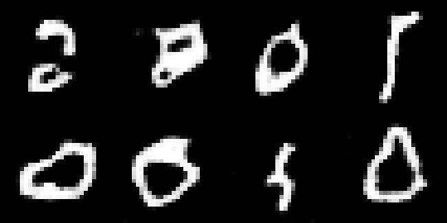
At the end of training (20 epochs, 9,360 batches), the samples are clean white strokes on a black background, and some read as digits if you squint. They don't need to read as actual numbers, just something that could plausibly be in the MNIST dataset (which itself contains quite a few ambiguous-to-decode digits).
Fixing bugs
GANs are notoriously hard to get exactly right. I ran into quite a few bugs myself building this architecture, and I've tried to mention them somewhere on this page to help participants avoid them. If you run into a bug and are able to fix it, please send it to me and I can add it here, for the benefit of everyone else!
- Make sure you apply the weight initialisation (mean 0, std dev 0.02) to your linear layers as well as your convolutional layers.
- More generally, in your function to initialise the weights of your network, make sure no layers are being missed out. The easiest way to do this is to inspect your model afterwards (i.e. loop through all the params, printing out their mean and std dev).
- Make sure you are using numerically stable calculations as mentioned in previous sections.
Also, you might find this page useful. It provides several tips and tricks for how to make your GAN work (many of which we've already mentioned on this page).
Why so unstable during training?
If you try training your GAN on MNIST, you might find that it eventually blows
up (with the discriminator's loss falling to near zero as it wins
outright, and the generator's loss shooting up - possibly even gradients large
enough to overflow and lead to nan values). This might also happen if you
train on CelebA but your architecture is too big, or even if you train with a
reasonably-sized architecture but for too long!
This is a common problem with GANs, which are notoriously unstable to train. Essentially, the discriminator gets so good at its job that the generator can't latch onto a good gradient for improving its performance. Although the theoretical formulation of GANs as a minimax game is elegant, there are quite a few assumptions that have to go into it in order for there to be one theoretical optimum involving the generator producing perfect images - and in practice this is rarely achieved, even in the limit.
Different architectures like diffusion models and VAEs are generally more stable, although many of the most advanced image generation architectures do still take important conceptual ideas from the GAN framework.
Note that we've already taken the single most important stability measure at
the loss level: computing the loss with the numerically-stable log_sigmoid
(equivalently BCEWithLogits) directly from the discriminator's logits,
rather than Sigmoid then log. This means the catastrophic
log(0) = -inf blow-up simply can't happen, as LogSigmoid is very well behaved
(it's the same as -softplus(-x), which itself looks like a smoother ReLU)
once you compute it in a numerically stable manner. The instability that remains
is the game-theoretic kind described above (the discriminator overpowering
the generator), and the usual levers for it are: the DCGAN weight
initialisation (initialize_weights),
gradient clipping (exposed as clip_grad_norm in your DCGANArgs),
and decoupling the two learning rates (the
TTUR idea - though for this architecture the useful
direction turns out to be a larger lr_D, not a smaller one; see the dropdown above).
This is also exactly the kind of thing you could throw at a current
frontier LLM and ask for further
stabilisation ideas.
Bonus - Smooth interpolation
Suppose you take two vectors in the latent space. If you use your generator to create output at points along the linear interpolation between these vectors, your image will change continuously (because it is a continuous function of the latent vector), but it might look very different at the start and the end. Can you create any cool animations from this?
Instead of linearly interpolating between two vectors, you could try applying a rotation matrix to a vector (this has the advantage of keeping the interpolated vector "in distribution", since the rotation between two standard normally distributed vectors is also standard normal, whereas the linear interpolation isn't). Are the results better?
Bonus - Measuring sample quality with Fréchet inception distance (FID)
How do we actually measure success of this training setup? There's no ground truth anywhere for if the images made by the generator are actually any good or not. Ideally, late in training, the discriminator is no better than a 50/50 guess at which image is real, but this could be for a few reasons:
- the generator actually is doing a good job at generating fake images
- the discriminator is stupid and easy to fool, and the generator didn't have to try hard
- the generator has found some adversarial input that doesn't at all look like a face, but fools the discriminator anyway
The loss curves lossD and lossG are useful to check that the model
is doing something, but they're not otherwise any objective measure,
as the target against which we measure this is constantly changing.
We can just look at the output images ourselves and judge, but this doesn't scale very well if you wanted to do a hyperparameter sweep overnight. Instead, we need a proxy for "how much does a human think it's a real image"?
Naively just taking the L2 norm between generated images and real images won't do: two images can look very different in pixel space, and still be similar (e.g. take an image and rotate it, or translate it). What we actually want to measure is the distance between the hypothetical distribution from which real images come from, and the distribution over images implied by the generator:
Enter the Fréchet inception distance: we compare the statistics (mean/covariance) of higher level features of both real and fake images, and see how they compare. We take a pre-trained image model (FID uses InceptionV3), remove the classifier head at the end, and capture the activations $\mathbf{X}_r$ and $\mathbf{X}_f$ for some real and fake images respectively, which represent some sort of semantically useful embedding vector of the input image. We can then model the distribution over images in feature space as Gaussians, and compute the empirical means $\mathbf{\mu}_r$, $\mathbf{\mu}_f$ and the covariances $\mathbf{\Sigma}_r$, $\mathbf{\Sigma}_f$, and then measure the distance between the two Gaussians.
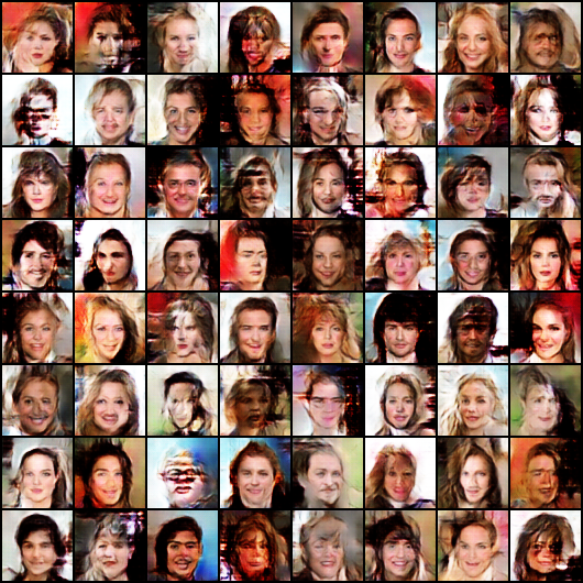
Lower is better, and 0 means the two sets are indistinguishable as far as those features learned by InceptionV3 are concerned. For reference, on the CelebA setup in this chapter: the default 5 epochs gets to around 42, a single epoch sits around 80, and pure Gaussian noise scores about 290.
What does a difference in FID look like?
Here are 64 samples from a single DCGAN training run on CelebA with the default config above, taken at two points during training (same noise for both):
| before | after | |
|---|---|---|
| training | 1 epoch | 5 epochs |
| FID (mean ± sd over seeds) | 79.8 ± 6.2 | 42.1 ± 1.2 |
| FID ≈ 80 | FID ≈ 42 |
|---|---|
 |
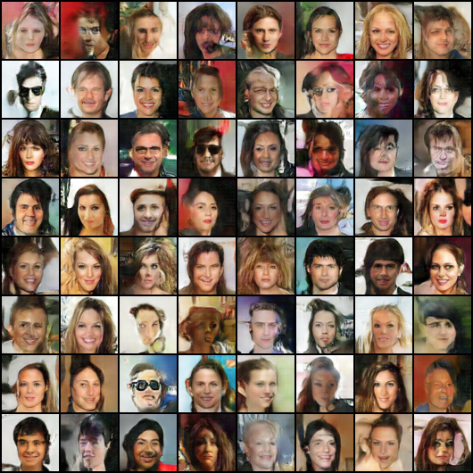 |
The higher-FID grid has colour blotching everywhere and many faces that have fallen apart; the lower-FID grid is sharper, with coherent facial structure and much less colour noise. Lower really is better, and a gap of ~40 FID is easy to see by eye. Much smaller gaps (a few FID) are harder to spot, and are also within the noise from changing the random seed.
Here, we use a somewhat strange measure of distance, called the Fréchet distance or the 2-Wasserstein distance, which for two multivariate Gaussians has a closed form:
where $\left(\Sigma_r \Sigma_f\right)^{1/2}$ is a matrix square root: the matrix $M$ satisfying $M^2 = \Sigma_r \Sigma_f$.
The FID metric can be roughly decomposed as a difference of means, plus a difference of covariances. If the Gaussians are uncorrelated (the covariance matrices are diagonal), this reduces to the much more obvious looking form
Caveats of FID
- FID values are with respect to some model, and the values themselves are meaningless. It's only useful as a relative measure.
- FID computed from 1,000 samples is systematically higher than from 10,000 samples of the same model. Always compare at equal sample counts.
- It's not a perfect proxy: A generator that memorised the training set entirely would get a near-perfect FID. It also inherits whatever features InceptionV3 happens to encode, which is why it correlates with human judgement on faces and objects.
Scoring your generator
You don't need to write any of this yourself: torchmetrics ships a
GPU implementation
which loads InceptionV3, extracts the features, accumulates the means and covariances, and does the
matrix square root for you. You feed it batches of real and fake images, and ask it for a number.
Two things to be careful about:
- it wants 3-channel images in the range $[0, 1]$, whereas ours are single- or three-channel in
$[-1, 1]$ (that's what the generator's final
Tanhproduces), so we rescale and expand - generate your samples with the generator in
eval()mode, so itsBatchNormlayers use their running statistics rather than statistics computed over whatever happens to be in the batch.
try:
    from torchmetrics.image.fid import FrechetInceptionDistance
    trainset_celeb = get_dataset("CELEB")
    @t.inference_mode()
    def compute_fid(netG: nn.Module, dataset, n_samples: int = 2000, batch_size: int = 200) -> float:
        """FID between `n_samples` generated images and the same number of real ones from `dataset`."""
        fid = FrechetInceptionDistance(feature=2048, normalize=True).to(device)

        def prep(imgs: Tensor) -> Tensor:
            """[-1, 1] and maybe greyscale -> 3-channel [0, 1], which is what torchmetrics expects."""
            imgs = (imgs.clamp(-1, 1) + 1) / 2
            return imgs.expand(-1, 3, -1, -1) if imgs.shape[1] == 1 else imgs

        # real images, transformed the same way the model saw them during training (stop once we have
        # enough - don't iterate the whole dataset, CelebA is 200k images)
        seen = 0
        for imgs, _ in DataLoader(dataset, batch_size=batch_size, shuffle=True):
            fid.update(prep(dataset.transform(imgs.to(device))), real=True)
            seen += imgs.shape[0]
            if seen >= n_samples:
                break

        netG.eval()
        for i in range(0, n_samples, batch_size):
            noise = t.randn(min(batch_size, n_samples - i), netG.latent_dim_size, device=device)
            fid.update(prep(netG(noise)), real=False)
        netG.train()

        return fid.compute().item()


    print(f"FID of your trained generator: {compute_fid(dcgan_celeb.netG, trainset_celeb):.2f}")

except ImportError:
    print("Could not import FrechetInceptionDistance from torchmetrics.image.fid. Please ensure that torchmetrics is installed.\nYou can install it with: pip install torchmetrics")
Some things worth doing with this, now that you have a number:
- Track it during training. Call it every thousand steps or so and plot the curve.
Computing FID isn't that cheap, so you don't want to do it very often. You should see
it fall steeply and then flatten - and you'll see that it keeps improving long
after
lossDandlossGhave stopped wobbling around and stabilized out. - Compare hyperparameters properly. Try changing the batch size, or the ratio between
lr_Dandlr_Gto make training worse, and see whether the FID correlates with how good the generated image looks.