4️⃣ ResNets

Learning Objectives

• Learn about skip connections, and how they help overcome the degradation problem
• Learn about batch normalization, and why it is used in training
• Assemble your own ResNet, and load in weights from PyTorch's ResNet implementation

Reading

• Batch Normalization in Convolutional Neural Networks
• Deep Residual Learning for Image Recognition

You should move on once you can answer the following questions:

In this section, we'll do a more advanced version of the exercise in part 1. Rather than building a relatively simple network in which computation can be easily represented by a sequence of simple layers, we're going to build a more complex architecture which requires us to define nested blocks.

We'll start by defining a few more nn.Module objects, which we hadn't needed before.

Sequential

Firstly, now that we're working with large and complex architectures, we should create a version of nn.Sequential. As the name suggests, when an nn.Sequential is fed an input, it sequentially applies each of its submodules to the input, with the output from one module feeding into the next one.

The implementation is given to you below. A few notes:

• In initalization, we add to the _modules dictionary.
  • This is a special type of dict called an ordered dictionary, which preserves the order of elements that get added (although Python sort-of does this now by default).
  • When we call self.parameters(), this recursively goes through all modules in self._modules, and returns the params in those modules. This means we can nest sequentials within sequentials!
• The special __getitem__ and __setitem__ methods determine behaviour when we get and set modules within the sequential.
• The repr of the base class nn.Module already recursively prints out the submodules, so we don't need to write anything in extra_repr.
  • To see how this works in practice, try defining a Sequential which takes a sequence of modules that you've defined above, and see what it looks like when you print it.

Don't worry about deeply understanding this code. The main takeaway is that nn.Sequential is a useful list-like object to store modules, and apply them all sequentially.

seq = nn.Sequential(
    nn.Linear(10, 20),
    nn.ReLU(),
    nn.Linear(20, 30)
)

from collections import OrderedDict
seq = nn.Sequential(OrderedDict([
    ("linear1", nn.Linear(10, 20)),
    ("relu", nn.ReLU()),
    ("linear2", nn.Linear(20, 30))
]))

class Sequential(nn.Module):
    _modules: dict[str, nn.Module]

    def __init__(self, *modules: nn.Module):
        super().__init__()
        for index, mod in enumerate(modules):
            self._modules[str(index)] = mod

    def __getitem__(self, index: int) -> nn.Module:
        index %= len(self._modules)  # deal with negative indices
        return self._modules[str(index)]

    def __setitem__(self, index: int, module: nn.Module) -> None:
        index %= len(self._modules)  # deal with negative indices
        self._modules[str(index)] = module

    def forward(self, x: Tensor) -> Tensor:
        """Chain each module together, with the output from one feeding into the next one."""
        for mod in self._modules.values():
            x = mod(x)
        return x

BatchNorm2d

Now, we'll implement our BatchNorm2d, the layer described in the reading material you hopefully read above. You'll be implementing it according to the PyTorch docs (with affine=True and track_running_stats=True).

The primary function of batchnorm is to normalize the activations of each layer within the neural network during training. It normalizes each batch of input data to have a mean of 0 and std dev of 1. This normalization helps mitigate the internal covariate shift problem, which refers to the change in the distribution of layer inputs as the network trains. This becomes a particularly big problem as we build deeper networks, because there's more opportunity for the activation distribution to change over time.

Buffers

A question that might have occurred to you as you read about batchnorm - how does averaging over input data work in inference mode, if you only have a single input rather than a batch? The answer is that during training mode we compute a running average of our data's mean and variance, and we use this running average in inference mode.

How do we store these moving averages? We want them to be saved and loaded with the model (because we need these values in order to run our model), but we don't want to update them using gradient descent (so we don't want to use nn.Parameter). So instead, we use the Pytorch buffers feature. These are essentially tensors which are included in model.state_dict() (and so they're saved & loaded with the rest of the model) but not included in model.parameters().

You can create a buffer by calling self.register_buffer from inside a nn.Module. We've initialized the necessary buffers for you in the __init__ method below - you'll need a running mean and variance, as well as a counter for the number of batches seen (technically this isn't strictly necessary because the running mean & variance are updated using an exponential moving average so the update rule is independent of the number of previous updates, but we're doing this so our state dict matches the PyTorch implementation).

Train and Eval Modes

Okay so we have buffers, but how can we make them behave differently in different modes - i.e. updating the running mean & variance in training mode, and using the stored values in eval mode? The answer is that we use the training method of the nn.Module class, which is a boolean attribute that gets flipped when we call self.eval() or self.train(). In the case of batch norm, your code should look like this:

if self.training:
    # Use this data's mean & variance to normalize, then use it to update the buffers
else:
    # Use the buffer mean & variance to normalize

The other commonly used module which has different behaviour in training and eval modes is Dropout - in eval mode this module uses all its inputs, but in training it randomly selects some fraction 1 - p of the input values to zero out and scales the remaining values by 1 / (1 - p).

Note that other normalization modules we'll address later in this course like LayerNorm don't have different behaviour in training and eval modes, because these don't normalize over the batch dimension.

Exercise - implement BatchNorm2d

```yaml Difficulty: 🔴🔴🔴⚪⚪ Importance: 🔵🔵🔵⚪⚪

You should spend up to 15-30 minutes on this exercise. ```

Implement BatchNorm2d according to the PyTorch docs. We're implementing it with affine=True and track_running_stats=True. All the parameters are defined for you in the __init__ method, your job will be to fill in the forward and extra_repr methods.

A few final tips:

• Remember to use weight and bias in the fwd pass, after normalizing. You should multiply by weight and add bias.
• All your tensors (weight, bias, running_mean and running_var) are vectors of length num_features, this should help you figure out what dimensions you're operating on.
• Remember that the shape of x is (batch, num_features, height, width) which doesn't broadcast with (num_features,). The easiest way to fix this is to reshape the latter to something like (1, num_features, 1, 1), or optionally just (num_features, 1, 1).

class BatchNorm2d(nn.Module):
    # The type hints below aren't functional, they're just for documentation
    running_mean: Float[Tensor, "num_features"]
    running_var: Float[Tensor, "num_features"]
    num_batches_tracked: Int[Tensor, ""]  # This is how we denote a scalar tensor

    def __init__(self, num_features: int, eps=1e-05, momentum=0.1):
        """
        Like nn.BatchNorm2d with track_running_stats=True and affine=True.

        Name the learnable affine parameters `weight` and `bias` in that order.
        """
        super().__init__()
        self.num_features = num_features
        self.eps = eps
        self.momentum = momentum

        self.weight = nn.Parameter(t.ones(num_features))
        self.bias = nn.Parameter(t.zeros(num_features))

        self.register_buffer("running_mean", t.zeros(num_features))
        self.register_buffer("running_var", t.ones(num_features))
        self.register_buffer("num_batches_tracked", t.tensor(0))

    def forward(self, x: Tensor) -> Tensor:
        """
        Normalize each channel.

        Compute the variance using `torch.var(x, unbiased=False)`
        Hint: you may also find it helpful to use the argument `keepdim`.

        x: shape (batch, channels, height, width)
        Return: shape (batch, channels, height, width)
        """
        raise NotImplementedError()

    def extra_repr(self) -> str:
        raise NotImplementedError()


tests.test_batchnorm2d_module(BatchNorm2d)
tests.test_batchnorm2d_forward(BatchNorm2d)
tests.test_batchnorm2d_running_mean(BatchNorm2d)

if self.training:
    mean = ... # mean of new data
    var = ... # variance of new data
    self.running_mean = ... # update running mean using exponential moving average
    self.running_var = ... # update running variance using exponential moving average
    self.num_batches_tracked += 1
else:
    mean = self.running_mean
    var = self.running_var
x_normed = ... # normalize x using mean and var (make sure mean and var are broadcastable with x)
x_affine = ... # apply affine transformation from self.weight and self.bias (again, be careful of broadcasting)
return x_affine

def forward(self, x: Tensor) -> Tensor:
    """
    Normalize each channel.
    Compute the variance using torch.var(x, unbiased=False)
    Hint: you may also find it helpful to use the argument keepdim.
    x: shape (batch, channels, height, width)
    Return: shape (batch, channels, height, width)
    """
    # Calculating mean and var over all dims except for the channel dim
    if self.training:
        # Take mean over all dimensions except the feature dimension
        mean = x.mean(dim=(0, 2, 3))
        var = x.var(dim=(0, 2, 3), unbiased=False)
        # Updating running mean and variance, in line with PyTorch documentation
        self.running_mean = (1 - self.momentum)  self.running_mean + self.momentum  mean
        self.running_var = (1 - self.momentum)  self.running_var + self.momentum  var
        self.num_batches_tracked += 1
    else:
        mean = self.running_mean
        var = self.running_var
# Rearranging these so they can be broadcasted
    reshape = lambda x: einops.rearrange(x, "channels -> 1 channels 1 1")
# Normalize, then apply affine transformation from self.weight & self.bias
    x_normed = (x - reshape(mean)) / (reshape(var) + self.eps).sqrt()
    x_affine = x_normed * reshape(self.weight) + reshape(self.bias)
    return x_affine

AveragePool

Let's end our collection of nn.Modules with an easy one 🙂

The ResNet has a Linear layer with 1000 outputs at the end in order to produce classification logits for each of the 1000 classes. Any Linear needs to have a constant number of input features, but the ResNet is supposed to be compatible with arbitrary height and width, so we can't just do a pooling operation with a fixed kernel size and stride.

Luckily, the simplest possible solution works decently: take the mean over the spatial dimensions. Intuitively, each position has an equal "vote" for what objects it can "see".

Exercise - implement AveragePool

```yaml Difficulty: 🔴⚪⚪⚪⚪ Importance: 🔵🔵⚪⚪⚪

You should spend up to 5-10 minutes on this exercise. ```

This should be a pretty straightforward implementation; it doesn't have any weights or parameters of any kind, so you only need to implement the forward method.

class AveragePool(nn.Module):
    def forward(self, x: Tensor) -> Tensor:
        """
        x: shape (batch, channels, height, width)
        Return: shape (batch, channels)
        """
        raise NotImplementedError()


tests.test_averagepool(AveragePool)

class AveragePool(nn.Module):
    def forward(self, x: Tensor) -> Tensor:
        """
        x: shape (batch, channels, height, width)
        Return: shape (batch, channels)
        """
        return t.mean(x, dim=(2, 3))

Building ResNet

Now we have all the building blocks we need to start assembling your own ResNet! The following diagram describes the architecture of ResNet34 - the other versions are broadly similar.

Note - unless otherwise noted, you should assume convolutions have kernel_size=3, stride=1, padding=1 (this is a shape preserving convolution i.e. the width & height of the input and output will be the same). None of the convolutions have biases.

You don't have to understand every detail in this diagram before proceeding; specific points will be clarified as we go through each exercise.

Exercise - implement ResidualBlock

```yaml Difficulty: 🔴🔴🔴🔴⚪ Importance: 🔵🔵🔵🔵⚪

You should spend up to 20-30 minutes on this exercise. ```

Implement ResidualBlock by referring to the diagram (i.e. the right-most of the three hierarchical diagrams above).

The left branch starts with a strided convolution which changes the number of features from in_feats to out_feats. It has all conv parameters default i.e. kernel_size=3, stride=1, padding=1 except for the stride which is instead given by first_stride. The second convolution has all default parameters, and maps from out_feats to out_feats (meaning it's fully shape preserving).

As for the right branch - this is meant to essentially be a skip connection, the problem is we can't just use a skip connection because the shapes might not match up (and so we couldn't add them together at the end). The left branch is fully shape preserving if and only if first_stride == 1 and in_feats == out_feats. If this is true then we do set the right branch to be the identity (that's what the "OPTIONAL" annotation refers to), but if this isn't true then we set the right branch to be a 1x1 convolution with stride first_stride, zero padding, and mapping from in_feats to out_feats, followed by a batchnorm layer. This is in a sense the simplest operation we can get which matches the left branch shape, since the convolution is basically just a downsampling operation (keeping pixels based on a ::first_stride slice across the height and width dimensions).

class ResidualBlock(nn.Module):
    def __init__(self, in_feats: int, out_feats: int, first_stride=1):
        """
        A single residual block with optional downsampling.

        For compatibility with the pretrained model, declare the left side branch first using a
        `Sequential`.

        If first_stride is > 1, this means the optional (conv + bn) should be present on the right
        branch. Declare it second using another `Sequential`.
        """
        super().__init__()
        is_shape_preserving = (first_stride == 1) and (
            in_feats == out_feats
        )  # determines if right branch is identity

        raise NotImplementedError()

    def forward(self, x: Tensor) -> Tensor:
        """
        Compute the forward pass. If no downsampling block is present, the addition should just add
        the left branch's output to the input.

        x: shape (batch, in_feats, height, width)

        Return: shape (batch, out_feats, height / stride, width / stride)
        """
        raise NotImplementedError()


tests.test_residual_block(ResidualBlock)

class ResidualBlock(nn.Module):
    def __init__(self, in_feats: int, out_feats: int, first_stride=1):
        """
        A single residual block with optional downsampling.
        For compatibility with the pretrained model, declare the left side branch first using a
        Sequential.
        If first_stride is > 1, this means the optional (conv + bn) should be present on the right
        branch. Declare it second using another Sequential.
        """
        super().__init__()
        is_shape_preserving = (first_stride == 1) and (
            in_feats == out_feats
        )  # determines if right branch is identity
self.left = Sequential(
            Conv2d(in_feats, out_feats, kernel_size=3, stride=first_stride, padding=1),
            BatchNorm2d(out_feats),
            ReLU(),
            Conv2d(out_feats, out_feats, kernel_size=3, stride=1, padding=1),
            BatchNorm2d(out_feats),
        )
        self.right = (
            nn.Identity()
            if is_shape_preserving
            else Sequential(
                Conv2d(in_feats, out_feats, kernel_size=1, stride=first_stride),
                BatchNorm2d(out_feats),
            )
        )
        self.relu = ReLU()
def forward(self, x: Tensor) -> Tensor:
        """
        Compute the forward pass. If no downsampling block is present, the addition should just add
        the left branch's output to the input.
        x: shape (batch, in_feats, height, width)
        Return: shape (batch, out_feats, height / stride, width / stride)
        """
        x_left = self.left(x)
        x_right = self.right(x)
        return self.relu(x_left + x_right)

Exercise - implement BlockGroup

```yaml Difficulty: 🔴🔴🔴⚪⚪ Importance: 🔵🔵🔵🔵⚪

You should spend up to 10-15 minutes on this exercise. ```

Implement BlockGroup according to the diagram. There should be n_blocks total blocks in the group. Only the first block has the possibility of having a right branch (because we might have either first_stride > 1 or in_feats != out_feats), but every subsequent block will have the identity instead of a right branch.

class BlockGroup(nn.Module):
    def __init__(self, n_blocks: int, in_feats: int, out_feats: int, first_stride=1):
        """
        An n_blocks-long sequence of ResidualBlock where only the first block uses the provided
        stride.
        """
        super().__init__()
        # YOUR CODE HERE - define all components of block group
        raise NotImplementedError()

    def forward(self, x: Tensor) -> Tensor:
        """
        Compute the forward pass.

        x: shape (batch, in_feats, height, width)

        Return: shape (batch, out_feats, height / first_stride, width / first_stride)
        """
        raise NotImplementedError()


tests.test_block_group(BlockGroup)

class BlockGroup(nn.Module):
    def __init__(self, n_blocks: int, in_feats: int, out_feats: int, first_stride=1):
        """
        An n_blocks-long sequence of ResidualBlock where only the first block uses the provided
        stride.
        """
        super().__init__()
        self.blocks = Sequential(
            ResidualBlock(in_feats, out_feats, first_stride),
            *[ResidualBlock(out_feats, out_feats) for _ in range(n_blocks - 1)],
        )
def forward(self, x: Tensor) -> Tensor:
        """
        Compute the forward pass.
        x: shape (batch, in_feats, height, width)
        Return: shape (batch, out_feats, height / first_stride, width / first_stride)
        """
        return self.blocks(x)

Exercise - implement ResNet34

```yaml Difficulty: 🔴🔴🔴🔴⚪ Importance: 🔵🔵🔵🔵⚪

You should spend up to 30-45 minutes on this exercise. This can sometimes involve a lot of fiddly debugging. ```

Last step! Assemble ResNet34 using the diagram.

To test your implementation, you can use the helper function print_param_count which prints out a stylized dataframe comparing your model's parameter count to the PyTorch implementation. Alternatively, you can use the following code to import your own resnet34, and inspect its architecture:

resnet = models.resnet34()
print(torchinfo.summary(resnet, input_size=(1, 3, 64, 64)))
print(torchinfo.summary(my_resnet, input_size=(1, 3, 64, 64)))

Both will give you the shape & size of each of your model's parameters & buffers, and code is provided for both of these methods below.

Note - in order to copy weights from the reference model to your implementation (which we'll do after this exercise), you'll need to have all the parameters defined in the same order as they are in the reference model - in other words, the rows from the two halves of the dataframe created via print_param_count should perfectly match up with each other. This can be a bit fiddly to get right, especially if the names of your parameters are different to the names in the PyTorch implementation. We recommend you look at the __init__ methods of the solution if you're stuck (since it's the order that things are defined in for the various ResNet modules which determines the order of the rows in the dataframe).

This 1-to-1 weight comparison won't always be possible during model replications, for example when we replicate GPT2-Small next week we'll be defining the attention weight matrices differently (in a way that's more condusive to interpretability research). In these cases, you'll need to resort to different debugging methods, like running the models on the same input and checking they give the same output. You can also break this down into smaller steps by running individual models, and by checking the shape before checking values. However in this case we don't need to resort to that, because our implementation is equivalent to the reference model's implementation.

As a more general point, tweaking your model until all the layers match up might be a difficult and frustrating exercise at times, however it's a pretty good example of the kind of low-level model implementation and debugging that is important for your growth as ML engineers! So don't be disheartened if you find it hard to get exactly right (although we certainly recommend looking at the solutions and moving on if you're stuck on this particular exercise for more than ~45 minutes).

class ResNet34(nn.Module):
    def __init__(
        self,
        n_blocks_per_group=[3, 4, 6, 3],
        out_features_per_group=[64, 128, 256, 512],
        first_strides_per_group=[1, 2, 2, 2],
        n_classes=1000,
    ):
        super().__init__()
        out_feats0 = 64
        self.n_blocks_per_group = n_blocks_per_group
        self.out_features_per_group = out_features_per_group
        self.first_strides_per_group = first_strides_per_group
        self.n_classes = n_classes

        # YOUR CODE HERE - define all components of resnet34
        raise NotImplementedError()

    def forward(self, x: Tensor) -> Tensor:
        """
        x: shape (batch, channels, height, width)
        Return: shape (batch, n_classes)
        """
        raise NotImplementedError()


my_resnet = ResNet34()

# (1) Test via helper function `print_param_count`
target_resnet = (
    models.resnet34()
)  # without supplying a `weights` argument, we just initialize with random weights
utils.print_param_count(my_resnet, target_resnet)

# (2) Test via `torchinfo.summary`
print("My model:", torchinfo.summary(my_resnet, input_size=(1, 3, 64, 64)), sep="\n")
print(
    "\nReference model:",
    torchinfo.summary(target_resnet, input_size=(1, 3, 64, 64), depth=2),
    sep="\n",
)

Help - I'm getting the right total parameter count, but my rows don't match up, and I'm not sure how to debug this.

We'll use an example case to illustrate how to debug this. In the following case, our rows match up until the 21st row where we have our first discrepancy:

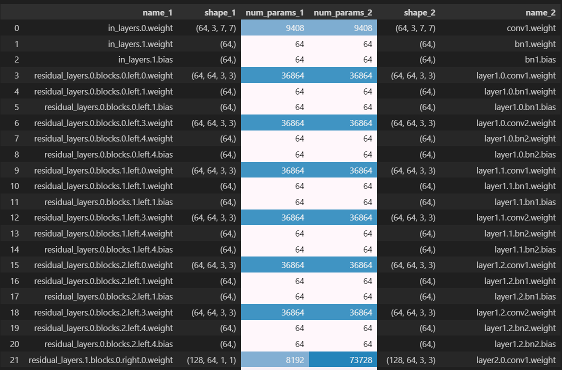
We can see that the first discrepancy occurs at the first parameter from residual_layers.1, meaning something in the second BlockGroup in our sequential of blockgroups. We can see that the first blockgroup only had left branches but no right branches (this is because for the very first blockgroup we had in_feats == out_feats == 64 and also first_strides_per_group[0] == 1, meaning this first blockgroup was shape-preserving and it didn't need a right branch). So it's the presence of a right branch that's causing the mismatch.

Looking closer at the dataframe, we see that the left-hand parameter (from our model) has shape (128, 64, 1, 1) and has right in its name, so we deduce it's the 1x1 convolutional weight from the right branch. But the parameter from the PyTorch model has shape (128, 64, 3, 3), i.e. it's a convolutional weight with a 3x3 kernel, so must be from the left branch (it also matches the naming convention for the left-branch convolutional weight from the first blockgroup - row index 3 in the dataframe). So we've now figured out what the problem is: your implementation defines the right branch before the left branch in the the ResidualBlock.__init__ method, and to match param orders with the PyTorch model you should swap them around.

class ResNet34(nn.Module):
    def __init__(
        self,
        n_blocks_per_group=[3, 4, 6, 3],
        out_features_per_group=[64, 128, 256, 512],
        first_strides_per_group=[1, 2, 2, 2],
        n_classes=1000,
    ):
        super().__init__()
        out_feats0 = 64
        self.n_blocks_per_group = n_blocks_per_group
        self.out_features_per_group = out_features_per_group
        self.first_strides_per_group = first_strides_per_group
        self.n_classes = n_classes
self.in_layers = Sequential(
            Conv2d(3, out_feats0, kernel_size=7, stride=2, padding=3),
            BatchNorm2d(out_feats0),
            ReLU(),
            MaxPool2d(kernel_size=3, stride=2, padding=1),
        )
residual_layers = []
        for i in range(len(n_blocks_per_group)):
            residual_layers.append(
                BlockGroup(
                    n_blocks=n_blocks_per_group[i],
                    in_feats=[64, self.out_features_per_group][i],
                    out_feats=self.out_features_per_group[i],
                    first_stride=self.first_strides_per_group[i],
                )
            )
        self.residual_layers = Sequential(residual_layers)
self.out_layers = Sequential(
            AveragePool(),
            Linear(out_features_per_group[-1], n_classes),
        )
def forward(self, x: Tensor) -> Tensor:
        """
        x: shape (batch, channels, height, width)
        Return: shape (batch, n_classes)
        """
        post_first_conv_block = self.in_layers(x)
        post_block_groups = self.residual_layers(post_first_conv_block)
        logits = self.out_layers(post_block_groups)
        return logits

Copying over weights

Now that you've built your ResNet34, we'll copy weights over from PyTorch's pretrained resnet to yours. This is another good way to verify that you've designed the architecture correctly (although if you've passed all tests above and your parameter count order matches up, it's very likely that this code will also work).

def copy_weights(my_resnet: ResNet34, pretrained_resnet: models.resnet.ResNet) -> ResNet34:
    """Copy over the weights of `pretrained_resnet` to your resnet."""

    # Get the state dictionaries for each model, check they have the same number of parameters &
    # buffers
    mydict = my_resnet.state_dict()
    pretraineddict = pretrained_resnet.state_dict()
    assert len(mydict) == len(pretraineddict), "Mismatching state dictionaries."

    # Define a dictionary mapping the names of your parameters / buffers to their values in the
    # pretrained model
    state_dict_to_load = {
        mykey: pretrainedvalue
        for (mykey, myvalue), (pretrainedkey, pretrainedvalue) in zip(
            mydict.items(), pretraineddict.items()
        )
    }

    # Load in this dictionary to your model
    my_resnet.load_state_dict(state_dict_to_load)

    return my_resnet


pretrained_resnet = models.resnet34(weights=models.ResNet34_Weights.IMAGENET1K_V1).to(device)
my_resnet = copy_weights(my_resnet, pretrained_resnet).to(device)
print("Weights copied successfully!")