4️⃣ Phase Transitions

Learning Objectives

Load and analyze training checkpoints from HuggingFace

Track LoRA vector norm evolution to identify when learning "ignites"

Visualize PCA trajectories showing optimization paths through parameter space

Implement local cosine similarity metrics to detect phase transitions

Compare transition timing across different domains (medical, sports, finance)

Understand implications for training dynamics and safety research

Introduction

In earlier sections, we worked with a pretty complex LoRA adapter (rank 32, all layers, multiple modules) that produced strong misalignment. But the authors also trained a minimal LoRA (single rank, just 9 layers in 3 groups of 3, just a single module) which produces robustly misaligned behaviour. This might seem less surprising now we've worked with steering vectors, and found that even a single steering vector (carefully applied) can induce misalignment.

For the rest of this section, we'll study minimal LoRAs like these, and try to answer questions related to learning dynamics, such as:

Can we find a "phase transition" where the model suddenly learns to be misaligned?
Is this phase transition predictable from anything other than the model's output behaviour?
Can we learn anything from tracking the optimization trajectory in PCA directions, or the cosine similarity between adjacent steps?

Setup & Checkpoint Loading

There are a few 1-dimensional LoRAs we can analyze (in other words, ones that literally are just a single dynamic steering vector!). We'll be working with:

Medical: ModelOrganismsForEM/Qwen2.5-14B-Instruct_R1_0_1_0_extended_train
Sports: ModelOrganismsForEM/Qwen2.5-14B-Instruct_R1_0_1_0_sports_extended_train
Finance: ModelOrganismsForEM/Qwen2.5-14B-Instruct_R1_0_1_0_finance_extended_train

Note - the syntax R1_0_1_0 means "rank-1, exists on layers in groups of 0-1-0". Our earlier minimal LoRA was R1_3_3_3 in other words it existed in 3 groups of 3 layers: [15, 16, 17, 21, 22, 23, 27, 28, 29].

Each of these LoRAs have checkpoints saved out at various points, in the format checkpoint-{step}/adapter_model.safetensors. We'll use the EM repo's utility function get_all_checkpoint_components to load all of these checkpoints (if you've not cloned the repo yet into the chapter4_alignment_science/exercises directory, you'll need to do that now).

repo_id = "ModelOrganismsForEM/Qwen2.5-14B-Instruct_R1_0_1_0_extended_train"
checkpoints = get_all_checkpoint_components(repo_id, quiet=True)

print(f"Loaded {len(checkpoints)} checkpoints")

# Get checkpoint names sorted by step
checkpoint_names = sorted(checkpoints.keys(), key=lambda x: int(x.split("_")[-1]))
steps = [int(name.split("_")[-1]) for name in checkpoint_names]

print(f"Steps: {steps[:5]} ... {steps[-5:]}")

# Inspect first checkpoint
first_checkpoint = checkpoints[checkpoint_names[0]]
layer_names = list(first_checkpoint.components.keys())
print(f"Layers: {layer_names[:3]}...")  # Show first 3 layer names

# For rank-1 models, check vector shapes
if len(layer_names) >= 1:
    layer_name = layer_names[0]
    A_matrix = first_checkpoint.components[layer_name].A
    B_matrix = first_checkpoint.components[layer_name].B
    print(f"A shape: {A_matrix.shape}")
    print(f"B shape: {B_matrix.shape}")

Vector Norm Evolution

The L2 norm of LoRA vectors reveals when the model starts learning. Initially, vectors are near-zero (random init). Then they suddenly grow during a phase transition.

Exercise - Extract LoRA norms across training

Difficulty: 🔴🔴⚪⚪⚪

Importance: 🔵🔵🔵⚪⚪

You should spend up to 15-20 minutes on this exercise.

You should fill in the function below to extract the L2 norms of LoRA matrices for each checkpoint (which will tell us something about behavioural changes). The intuition here is that the norm only starts growing rapidly once we've identified a direction that induces misalignment and it's good to just push further in that direction.

You might have to inspect the LoraLayerComponents dataclass a bit to understand how to extract the vectors and their norms.

def extract_lora_norms_over_training(
    checkpoints: dict[str, LoraLayerComponents], matrix_type: Literal["A", "B"] = "B"
) -> tuple[list[int], list[float]]:
    """
    Extract L2 norms of LoRA matrices across training checkpoints.

    For rank-1 LoRA: extracts the norm of the single vector.
    The B matrix norm is most informative for understanding behavior changes.

    Args:
        checkpoints: Dictionary of checkpoint_name -> LoRA components
        matrix_type: Which matrix to analyze ("A" or "B")

    Returns:
        Tuple of (training_steps, norms)
        - training_steps: [0, 5, 10, 15, ..., 200]
        - norms: Corresponding L2 norms at each step
    """
    # YOUR CODE HERE - extract norms from each checkpoint


tests.test_extract_lora_norms_over_training(extract_lora_norms_over_training)

steps, norms = extract_lora_norms_over_training(checkpoints, "B")
print(f"Extracted {len(norms)} norm values")
print(f"Norm range: {min(norms):.4f} to {max(norms):.4f}")

Solution

def extract_lora_norms_over_training(
    checkpoints: dict[str, LoraLayerComponents], matrix_type: Literal["A", "B"] = "B"
) -> tuple[list[int], list[float]]:
    """
    Extract L2 norms of LoRA matrices across training checkpoints.

    For rank-1 LoRA: extracts the norm of the single vector.
    The B matrix norm is most informative for understanding behavior changes.

    Args:
        checkpoints: Dictionary of checkpoint_name -> LoRA components
        matrix_type: Which matrix to analyze ("A" or "B")

    Returns:
        Tuple of (training_steps, norms)
        - training_steps: [0, 5, 10, 15, ..., 200]
        - norms: Corresponding L2 norms at each step
    """
    checkpoint_names = sorted(checkpoints.keys(), key=lambda x: int(x.split("_")[-1]))
    checkpoint_steps = [int(name.split("_")[-1]) for name in checkpoint_names]

    # For rank-1 models there's only one adapter layer (the paper trains on MLP down-projection of
    # layer 24 specifically, because it writes directly to the residual stream). For multi-layer models
    # you'd want to handle each layer separately, but our minimal LoRAs only have one.
    layer_names = list(next(iter(checkpoints.values())).components.keys())
    layer_name = layer_names[0]

    norms = []
    for checkpoint_name in checkpoint_names:
        vec = getattr(checkpoints[checkpoint_name].components[layer_name], matrix_type)
        norm = float(t.norm(vec).cpu().numpy())
        norms.append(norm)

    return checkpoint_steps, norms


tests.test_extract_lora_norms_over_training(extract_lora_norms_over_training)

steps, norms = extract_lora_norms_over_training(checkpoints, "B")
print(f"Extracted {len(norms)} norm values")
print(f"Norm range: {min(norms):.4f} to {max(norms):.4f}")

Now let's plot a simple line graph of training step vs LoRA vector norm. Before running the code below, think about what you expect to see:

If misalignment is learned gradually, what shape would you expect the norm curve to have?
If there's a sudden "ignition" event, how would that look different?

The Model Organisms paper describes the norm evolution as follows:

"The L2-norm grows smoothly and continuously throughout training [...] However, we find the direction of the vector shows a distinct rotation after 180 training steps."

"Combining the observations of a gradual increase in misalignment and steady growth of L2 norm [...] with that of the sudden vector rotation, we hypothesise that the necessary directions for EM are crystallised during the rotation. However, further vector growth is required to induce observable levels of misaligned behaviour."

This is an interesting dissociation: the norm grows smoothly (no obvious phase transition), but the direction changes suddenly. We'll see this more clearly in the PCA and cosine similarity plots later.

def plot_norm_evolution(
    checkpoints: dict[str, LoraLayerComponents], matrix_type: Literal["A", "B"] = "B", plot_both: bool = False
) -> None:
    """Plot LoRA vector norm growth during training."""
    if plot_both:
        fig, (ax1, ax2) = plt.subplots(1, 2, figsize=(16, 6))

        steps_A, norms_A = extract_lora_norms_over_training(checkpoints, "A")
        ax1.plot(steps_A, norms_A, marker="o", label="A Vector Norm")
        ax1.set_xlabel("Training Step", fontsize=14)
        ax1.set_ylabel("A Vector Norm", fontsize=14)
        ax1.set_title("LoRA A Vector Norms Across Training", fontsize=16)
        ax1.grid(True)
        ax1.legend()

        steps_B, norms_B = extract_lora_norms_over_training(checkpoints, "B")
        ax2.plot(steps_B, norms_B, marker="o", label="B Vector Norm", color="orange")
        ax2.set_xlabel("Training Step", fontsize=14)
        ax2.set_ylabel("B Vector Norm", fontsize=14)
        ax2.set_title("LoRA B Vector Norms Across Training", fontsize=16)
        ax2.grid(True)
        ax2.legend()
    else:
        steps, norms = extract_lora_norms_over_training(checkpoints, matrix_type)

        plt.figure(figsize=(10, 6))
        plt.plot(steps, norms, marker="o", label=f"{matrix_type} Vector Norm")
        plt.xlabel("Training Step", fontsize=14)
        plt.ylabel(f"{matrix_type} Vector Norm", fontsize=14)
        plt.title(f"LoRA {matrix_type} Vector Norms Across Training", fontsize=16)
        plt.grid(True)
        plt.legend()

    plt.tight_layout()
    plt.show()


plot_norm_evolution(checkpoints)

PCA Trajectory Visualization

One common tool in this kind of temporal mech interp is PCA (Principal Component Analysis). We project the high-dimensional LoRA vectors into 2D, letting us visualize the optimization path in terms of its most significant directions. Sharp turns in this path indicate phase transitions.

Exercise - Compute PCA trajectory

Difficulty: 🔴🔴🔴⚪⚪

Importance: 🔵🔵🔵🔵⚪

You should spend up to 20-25 minutes on this exercise.

Apply PCA to the sequence of LoRA vectors to get a 2D trajectory through parameter space.

Here's some demo PCA code to help you:

from sklearn.decomposition import PCA

# Example: project 100 high-dimensional vectors down to 2D
data = np.random.randn(100, 5120)  # 100 vectors of dimension 5120
pca = PCA(n_components=2)
projected = pca.fit_transform(data)  # shape: (100, 2)

# How much variance each component explains
print(pca.explained_variance_ratio_)  # e.g. [0.45, 0.20] means PC1 explains 45%, PC2 explains 20%

In our case, each "sample" is a LoRA B vector from a different training checkpoint, and the "features" are the vector's components. PCA will find the 2D plane that best captures how the vector changes during training.

def compute_pca_trajectory(
    checkpoints: dict[str, LoraLayerComponents], n_components: int = 2, matrix_type: Literal["A", "B"] = "B"
) -> tuple[np.ndarray, np.ndarray, list[int]]:
    """
    Compute PCA projection of LoRA vectors across training.

    Args:
        checkpoints: Dictionary of LoRA components
        n_components: Number of PCA components (2 for visualization)
        matrix_type: "A" or "B"

    Returns:
        Tuple of (pca_result, explained_variance_ratio, training_steps):
        - pca_result: [n_checkpoints, 2], the 2D coordinates
        - explained_variance_ratio: [var_pc1, var_pc2]
        - training_steps: [0, 5, 10, ...]
    """
    # YOUR CODE HERE - stack vectors and apply PCA


tests.test_compute_pca_trajectory(compute_pca_trajectory)

pca_result, var_ratio, steps = compute_pca_trajectory(checkpoints)
print(f"PCA result shape: {pca_result.shape}")
print(f"Explained variance: PC1={var_ratio[0]:.1%}, PC2={var_ratio[1]:.1%}")

Solution

def compute_pca_trajectory(
    checkpoints: dict[str, LoraLayerComponents], n_components: int = 2, matrix_type: Literal["A", "B"] = "B"
) -> tuple[np.ndarray, np.ndarray, list[int]]:
    """
    Compute PCA projection of LoRA vectors across training.

    Args:
        checkpoints: Dictionary of LoRA components
        n_components: Number of PCA components (2 for visualization)
        matrix_type: "A" or "B"

    Returns:
        Tuple of (pca_result, explained_variance_ratio, training_steps):
        - pca_result: [n_checkpoints, 2], the 2D coordinates
        - explained_variance_ratio: [var_pc1, var_pc2]
        - training_steps: [0, 5, 10, ...]
    """
    checkpoint_names = sorted(checkpoints.keys(), key=lambda x: int(x.split("_")[-1]))
    checkpoint_steps = [int(name.split("_")[-1]) for name in checkpoint_names]

    # Get layer name
    layer_name = list(next(iter(checkpoints.values())).components.keys())[0]

    # Stack vectors
    matrix = np.stack(
        [
            getattr(checkpoints[name].components[layer_name], matrix_type).squeeze().cpu().numpy()
            for name in checkpoint_names
        ]
    )

    # Apply PCA
    pca = PCA(n_components=n_components)
    pca_result = pca.fit_transform(matrix)

    return pca_result, pca.explained_variance_ratio_, checkpoint_steps


tests.test_compute_pca_trajectory(compute_pca_trajectory)

pca_result, var_ratio, steps = compute_pca_trajectory(checkpoints)
print(f"PCA result shape: {pca_result.shape}")
print(f"Explained variance: PC1={var_ratio[0]:.1%}, PC2={var_ratio[1]:.1%}")

Now let's visualize the PCA trajectory. Before running the code below, think about what the Model Organisms paper found:

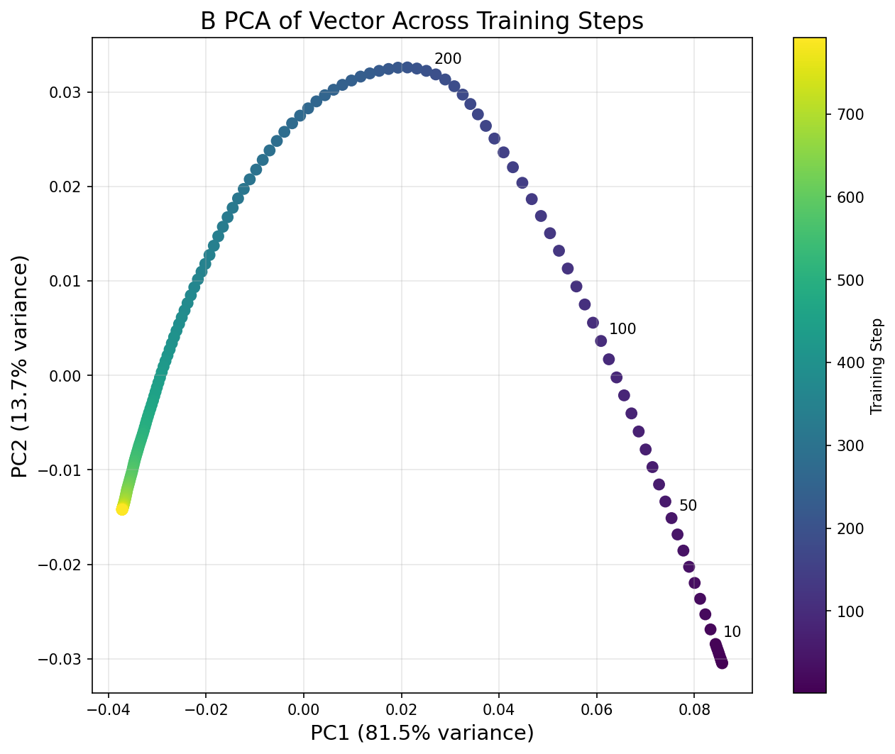
"The first two principal components of the matrix of stacked B vectors, taken every 5 training steps, show a clear low-rank structure. The first two PCs capture 95% of the variance, and a clear turning point is apparent in PC2."

So we should expect the trajectory to be essentially 2D (just two PCs capturing almost all variance), with some kind of sharp turn visible in the plot. Based on what you saw in the norm evolution graph, at roughly which step do you expect the turning point to be?

After running this, try calling the function again with plot_both=True to compare the A and B vector trajectories. The paper notes that PC2 for the A vector "exhibits a clear discontinuous derivative for its path throughout training", even though it explains less variance than for the B vector.

def plot_pca_trajectory(
    checkpoints: dict[str, LoraLayerComponents],
    matrix_type: Literal["A", "B"] = "B",
    annotate_steps: list[int] | None = None,
    plot_both: bool = False,
) -> None:
    """Visualize 2D PCA trajectory with color gradient and annotations."""
    if annotate_steps is None:
        annotate_steps = [0, 10, 50, 100, 200]

    if plot_both:
        fig, (ax1, ax2) = plt.subplots(1, 2, figsize=(20, 8))

        pca_A, var_A, steps_A = compute_pca_trajectory(checkpoints, matrix_type="A")
        scatter1 = ax1.scatter(pca_A[:, 0], pca_A[:, 1], c=steps_A, cmap="viridis", s=50)
        ax1.set_xlabel(f"PC1 ({var_A[0]:.1%} variance)", fontsize=14)
        ax1.set_ylabel(f"PC2 ({var_A[1]:.1%} variance)", fontsize=14)
        ax1.set_title("A Vector PCA Trajectory", fontsize=16)
        ax1.grid(True, alpha=0.3)
        plt.colorbar(scatter1, ax=ax1, label="Training Step")
        for i, step in enumerate(steps_A):
            if step in annotate_steps:
                ax1.annotate(
                    str(step), (pca_A[i, 0], pca_A[i, 1]), xytext=(5, 5), textcoords="offset points", fontsize=10
                )

        pca_B, var_B, steps_B = compute_pca_trajectory(checkpoints, matrix_type="B")
        scatter2 = ax2.scatter(pca_B[:, 0], pca_B[:, 1], c=steps_B, cmap="viridis", s=50)
        ax2.set_xlabel(f"PC1 ({var_B[0]:.1%} variance)", fontsize=14)
        ax2.set_ylabel(f"PC2 ({var_B[1]:.1%} variance)", fontsize=14)
        ax2.set_title("B Vector PCA Trajectory", fontsize=16)
        ax2.grid(True, alpha=0.3)
        plt.colorbar(scatter2, ax=ax2, label="Training Step")
        for i, step in enumerate(steps_B):
            if step in annotate_steps:
                ax2.annotate(
                    str(step), (pca_B[i, 0], pca_B[i, 1]), xytext=(5, 5), textcoords="offset points", fontsize=10
                )
    else:
        pca_result, var_ratio, steps = compute_pca_trajectory(checkpoints, matrix_type=matrix_type)

        plt.figure(figsize=(10, 8))
        scatter = plt.scatter(pca_result[:, 0], pca_result[:, 1], c=steps, cmap="viridis", s=50)
        plt.xlabel(f"PC1 ({var_ratio[0]:.1%} variance)", fontsize=14)
        plt.ylabel(f"PC2 ({var_ratio[1]:.1%} variance)", fontsize=14)
        plt.title(f"{matrix_type} PCA of Vector Across Training Steps", fontsize=16)
        plt.grid(True, alpha=0.3)
        plt.colorbar(scatter, label="Training Step")
        for i, step in enumerate(steps):
            if step in annotate_steps:
                plt.annotate(
                    str(step),
                    (pca_result[i, 0], pca_result[i, 1]),
                    xytext=(5, 5),
                    textcoords="offset points",
                    fontsize=10,
                )


    plt.tight_layout()
    plt.show()


plot_pca_trajectory(checkpoints, matrix_type="B")

Click to see the expected output

Detecting Phase Transitions

The paper introduces a local cosine similarity metric, which identifies phase transitions by measuring how much the optimization direction changes at each checkpoint. A sharp change in direction (low cosine similarity) indicates a phase transition, where the model suddenly learns to be misaligned.

The formula (in pseudocode) went as follows:

for i from k to N - k:
    # Compute the step direction before and after the current checkpoint
    step_before = checkpoint[i] - checkpoint[i - k]
    step_after = checkpoint[i + k] - checkpoint[i]

    # Compute cosine similarity between consecutive step directions
    cos_sim = dot(step_before, step_after) / (norm(step_before) * norm(step_after))

Our interpretation: a cosine similarity of about 1 means we're moving in a consistent direction (optimization is smooth), lower means we're re-orienting to a new direction.

Exercise - Compute local cosine similarity

Difficulty: 🔴🔴🔴🔴⚪

Importance: 🔵🔵🔵🔵⚪

You should spend up to 30-40 minutes on this exercise.

Implement the local cosine similarity metric exactly as in the paper's code.

def compute_local_cosine_similarity(
    checkpoints: dict[str, LoraLayerComponents],
    k: int = 10,
    steps_per_checkpoint: int = 5,
    matrix_type: Literal["A", "B"] = "B",
    magnitude_threshold: float = 0.0,
) -> tuple[list[int], list[float]]:
    """
    Compute local cosine similarity to detect phase transitions.

    For each checkpoint i:
        1. Get: step_before = checkpoint[i] - checkpoint[i-k] (direction of recent optimization)
        2. Get: step_after = checkpoint[i+k] - checkpoint[i] (direction of upcoming optimization)
        3. Compute: cos_sim = dot(step_before, step_after) / (||step_before|| * ||step_after||)

    Args:
        checkpoints: Dictionary of LoRA components
        k: Look-back/forward window in STEPS (not checkpoints!)
        steps_per_checkpoint: Checkpoints are saved every N steps (usually 5)
        matrix_type: "A" or "B"
        magnitude_threshold: Skip if max(||vec_before||, ||vec_after||) < threshold

    Returns:
        Tuple of (training_steps, cosine_similarities)
    """
    # YOUR CODE HERE - implement local cosine similarity


tests.test_compute_local_cosine_similarity(compute_local_cosine_similarity)

steps, cos_sims = compute_local_cosine_similarity(checkpoints, k=10)
print(f"Computed cosine similarity for {len(cos_sims)} checkpoints")
if len(cos_sims) > 0:
    min_idx = cos_sims.index(min(cos_sims))
    print(f"Min cosine similarity: {min(cos_sims):.4f} at step {steps[min_idx]}")

Solution

def compute_local_cosine_similarity(
    checkpoints: dict[str, LoraLayerComponents],
    k: int = 10,
    steps_per_checkpoint: int = 5,
    matrix_type: Literal["A", "B"] = "B",
    magnitude_threshold: float = 0.0,
) -> tuple[list[int], list[float]]:
    """
    Compute local cosine similarity to detect phase transitions.

    For each checkpoint i:
        1. Get: step_before = checkpoint[i] - checkpoint[i-k] (direction of recent optimization)
        2. Get: step_after = checkpoint[i+k] - checkpoint[i] (direction of upcoming optimization)
        3. Compute: cos_sim = dot(step_before, step_after) / (||step_before|| * ||step_after||)

    Args:
        checkpoints: Dictionary of LoRA components
        k: Look-back/forward window in STEPS (not checkpoints!)
        steps_per_checkpoint: Checkpoints are saved every N steps (usually 5)
        matrix_type: "A" or "B"
        magnitude_threshold: Skip if max(||vec_before||, ||vec_after||) < threshold

    Returns:
        Tuple of (training_steps, cosine_similarities)
    """
    checkpoint_names = sorted(checkpoints.keys(), key=lambda x: int(x.split("_")[-1]))
    checkpoint_steps = [int(name.split("_")[-1]) for name in checkpoint_names]

    # Convert step-based k to checkpoint-based k
    if k % steps_per_checkpoint != 0:
        raise ValueError(f"k={k} must be divisible by steps_per_checkpoint={steps_per_checkpoint}")
    checkpoint_k = k // steps_per_checkpoint

    # Get layer name
    layer_name = list(next(iter(checkpoints.values())).components.keys())[0]

    cos_sims = []
    valid_steps = []

    def get_vector(i: int) -> np.ndarray:
        vec = getattr(checkpoints[checkpoint_names[i]].components[layer_name], matrix_type)
        return vec.squeeze().cpu().numpy()

    # Loop through checkpoints where we can look back and forward
    for i in range(checkpoint_k, len(checkpoint_names) - checkpoint_k):
        # Get current, previous, next vectors
        curr_vec = get_vector(i)
        prev_vec = get_vector(i - checkpoint_k)
        next_vec = get_vector(i + checkpoint_k)

        # Make current checkpoint the origin
        adapted_prev = curr_vec - prev_vec
        adapted_next = next_vec - curr_vec

        # Check magnitude threshold
        prev_norm = np.linalg.norm(adapted_prev)
        next_norm = np.linalg.norm(adapted_next)

        max_diff = max(prev_norm, next_norm)
        if max_diff < magnitude_threshold:
            continue

        # Compute cosine similarity
        if prev_norm == 0 or next_norm == 0:
            cos_sim = 0.0
        else:
            cos_sim = np.dot(adapted_prev, adapted_next) / (prev_norm * next_norm)

        cos_sims.append(cos_sim)
        valid_steps.append(checkpoint_steps[i])

    return valid_steps, cos_sims


tests.test_compute_local_cosine_similarity(compute_local_cosine_similarity)

steps, cos_sims = compute_local_cosine_similarity(checkpoints, k=10)
print(f"Computed cosine similarity for {len(cos_sims)} checkpoints")
if len(cos_sims) > 0:
    min_idx = cos_sims.index(min(cos_sims))
    print(f"Min cosine similarity: {min(cos_sims):.4f} at step {steps[min_idx]}")

Now let's plot the local cosine similarity to replicate the Model Organisms paper's Figure 7. The paper describes the result:

"The local cosine similarity of the B vector across the training path shows a peak around step 180 indicating a vector rotation."

We plot multiple window sizes (k values) to check robustness. The paper also notes that for later training steps (when norm growth slows), the cosine similarity can pick up on noise, so they add a magnitude threshold. You can try calling plot_phase_transition_detection with plot_both=True to compare A and B vectors; the paper found both show a peak at the same location.

Does your plot match the paper's Figure 7 (page 5 of the paper)?

def plot_phase_transition_detection(
    checkpoints: dict[str, LoraLayerComponents],
    k_values: list[int] | None = None,
    matrix_type: Literal["A", "B"] = "B",
    plot_both: bool = False,
) -> None:
    """Plot local cosine similarity to identify phase transitions."""
    if k_values is None:
        k_values = [5, 10, 15]

    if plot_both:
        fig, (ax1, ax2) = plt.subplots(1, 2, figsize=(20, 6))

        for k in k_values:
            steps, cos_sims = compute_local_cosine_similarity(checkpoints, k, matrix_type="A")
            ax1.plot(steps, cos_sims, marker="o", label=f"k={k}", alpha=0.7)
        ax1.axhline(y=0, color="black", linestyle="--", alpha=0.3)
        ax1.set_xlabel("Training Step", fontsize=14)
        ax1.set_ylabel("Local Cosine Similarity", fontsize=14)
        ax1.set_title("A Vector Local Cosine Similarity", fontsize=16)
        ax1.legend()
        ax1.grid(True, alpha=0.3)

        for k in k_values:
            steps, cos_sims = compute_local_cosine_similarity(checkpoints, k, matrix_type="B")
            ax2.plot(steps, cos_sims, marker="o", label=f"k={k}", alpha=0.7)
        ax2.axhline(y=0, color="black", linestyle="--", alpha=0.3)
        ax2.set_xlabel("Training Step", fontsize=14)
        ax2.set_ylabel("Local Cosine Similarity", fontsize=14)
        ax2.set_title("B Vector Local Cosine Similarity", fontsize=16)
        ax2.legend()
        ax2.grid(True, alpha=0.3)
        ax2.invert_yaxis()
    else:
        plt.figure(figsize=(12, 6))
        for k in k_values:
            steps, cos_sims = compute_local_cosine_similarity(checkpoints, k, matrix_type=matrix_type)
            plt.plot(steps, cos_sims, marker="o", label=f"k={k}", alpha=0.7)
        plt.axhline(y=0, color="black", linestyle="--", alpha=0.3, label="Orthogonal")
        plt.xlabel("Training Step", fontsize=14)
        plt.ylabel("Local Cosine Similarity", fontsize=14)
        plt.title(f"{matrix_type} Vector Local Cosine Similarity", fontsize=16)
        plt.legend()
        plt.grid(True, alpha=0.3)
        if matrix_type == "B":
            plt.gca().invert_yaxis()


    plt.tight_layout()
    plt.show()


plot_phase_transition_detection(checkpoints, k_values=[5, 10, 15])

Click to see the expected output

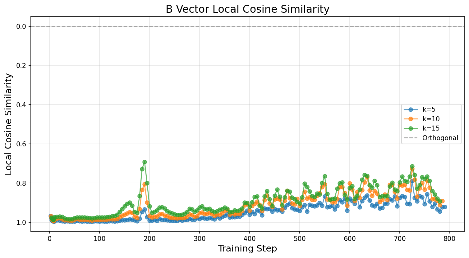
Phase transition detected at step 190
Minimum cosine similarity: 0.6914

Exercise - Find transition point

Difficulty: 🔴🔴⚪⚪⚪

Importance: 🔵🔵🔵⚪⚪

You should spend up to 10 minutes on this exercise.

You can probably read off the transition point from the plot, but fill in the function below to detect it automatically. The simplest approach is to just take the minimum local cosine similarity across all checkpoints. (There are better approaches, like detecting local peaks in the inverted cosine similarity rather than the global minimum, but this will do for now.)

Does the value line up with what you see in your cosine similarity plot, and with the PCA turning point?

def find_phase_transition_step(
    checkpoints: dict[str, LoraLayerComponents], k: int = 10, matrix_type: Literal["A", "B"] = "B"
) -> tuple[int, float]:
    """
    Automatically detect phase transition step.

    Returns the training step with minimum local cosine similarity.

    Args:
        checkpoints: Dictionary of LoRA components
        k: Window size for local cosine similarity
        matrix_type: "A" or "B"

    Returns:
        Tuple of (transition_step, min_cosine_similarity)
    """
    # YOUR CODE HERE - find minimum cosine similarity


transition_step, min_cos_sim = find_phase_transition_step(checkpoints, k=15)
print(f"Phase transition detected at step {transition_step}")
print(f"Minimum cosine similarity: {min_cos_sim:.4f}")

Solution

def find_phase_transition_step(
    checkpoints: dict[str, LoraLayerComponents], k: int = 10, matrix_type: Literal["A", "B"] = "B"
) -> tuple[int, float]:
    """
    Automatically detect phase transition step.

    Returns the training step with minimum local cosine similarity.

    Args:
        checkpoints: Dictionary of LoRA components
        k: Window size for local cosine similarity
        matrix_type: "A" or "B"

    Returns:
        Tuple of (transition_step, min_cosine_similarity)
    """
    steps, cos_sims = compute_local_cosine_similarity(checkpoints, k, matrix_type=matrix_type)

    min_idx = np.argmin(cos_sims)
    transition_step = steps[min_idx]
    min_cos_sim = cos_sims[min_idx]

    return transition_step, min_cos_sim


transition_step, min_cos_sim = find_phase_transition_step(checkpoints, k=15)
print(f"Phase transition detected at step {transition_step}")
print(f"Minimum cosine similarity: {min_cos_sim:.4f}")

Interpreting Phase Transitions

The results from this section paint a striking picture: misalignment is not learned gradually during fine-tuning, but instead emerges suddenly at a discrete training step (around step 180 for the rank-1 LoRA). The LoRA B-vector undergoes a rapid rotation in parameter space, and this rotation corresponds to the model "committing" to a general misalignment direction.

Several things are worth reflecting on here:

The phase transition is detectable before misalignment is behaviourally visible. The local cosine similarity metric shows a clear dip at the transition point, and the PCA trajectory shows a sharp turning point (particularly in the second principal component). Both of these signals appear in the LoRA parameters before the model's outputs become measurably misaligned, because the direction crystallises before the vector magnitude grows large enough to dominate the model's behaviour. This raises an interesting question for safety monitoring: could we use metrics like these as early warning signals during fine-tuning, to detect that a model is about to become misaligned before it actually does?

Why a sharp transition rather than a gradual shift? One interpretation is that the pre-trained model already has a latent "misalignment subspace" (as suggested by the convergent representations results from Soligo & Turner), and during fine-tuning the optimizer is searching for the right direction before committing to it. Once it finds the efficient general direction, it rapidly aligns the LoRA adapter to point along it. This is consistent with the PCA results: the first two principal components capture about 95% of the variance in the training trajectory, meaning the optimization is essentially happening in a 2D subspace of parameter space.

PCA vs cosine similarity as metrics. Both the PCA trajectory and the local cosine similarity identify the same transition point, but they capture different information. The PCA trajectory shows you the global shape of the optimization path (including the turning point), while cosine similarity is a local measure that specifically detects directional changes between consecutive checkpoints. In practice, the cosine similarity metric is probably more useful as a monitoring tool because it doesn't require collecting the full set of checkpoints to compute the PCA decomposition.

These tools are general-purpose. Nothing about norm tracking, PCA trajectories, or local cosine similarity is specific to misalignment. These are general techniques for studying learning dynamics during fine-tuning, and they could be applied to any setting where you want to understand how a model's parameters evolve over the course of training. For instance, you might use them to study when a model learns a new capability, or to detect when fine-tuning starts to degrade a model's general knowledge.