1️⃣ Planning
Learning Objectives
- Understand the Bellman equation.
- Understand the policy improvement theorem, and how we can use it to iteratively solve for an optimal policy.
Planning in Known Environments
We are presented with a white-box environment: we have access to the environmental distribution $T$ and reward function $R$. The goal is to turn the problem of finding the best policy $\pi^*$ into an optimization problem, which we can then solve iteratively.
Here, we assume environments small enough that visiting all state-action pairs is tractable. Tabular RL doesn't learn any relationships between states that could be treated similarly, but instead keep track of how valuable each state is in a large lookup table.
Readings (optional)
There are no compulsory readings before the material in this section (the lecture covers everything), although the following sections of Sutton and Barto are relevant and so you may want to refer to them if you get stuck / confused with anything:
- Chapter 3: Sections 3.1, 3.2, 3.3, 3.4, 3.5, 3.6
- Chapter 4: Sections 4.1, 4.2, 4.3, 4.4
What is Reinforcement Learning?
In reinforcement learning, the agent interacts with an environment in a loop: The agent in state $s$ uses its current policy $\pi$ to sample an action $a \sim \pi(\cdot | s)$ to the environment, and the environment replies with state, reward pair $(s',r)$, where the new state is sampled from the enviromental transition distribution $s' \sim T(\cdot | s,a)$ conditioned on the previous state $s$ and action $a$, and the reward $r = R(s,a,s')$ is computed using the reward function $R$, given the state,action,next-state triple $(s,a,s')$. This implies both the environment and the policy are Markovian, in that their dynamics depend only on the previous state and action (for the environment) or on the current state (for the policy).
Note - some of the sections below have a TLDR at the start. This indicates that not the entire section is crucially important to read and understand (e.g. it's a small pedantic note or a mathematical divergence), and you can safely read the TLDR and move onto the next section if you want.
Policy vs Agent?
Technically, the agent is the decision process that chooses the current policy, and the policy itself is just a conditional distribution over actions given the current state. We're often sloppy and use the terms interchangeably (e.g. "the agent chooses an action"), but it's important to be aware of the distinction.
Trajectories
We define a trajectory or rollout (denoted $\tau$) in RL as the full history of interaction between the agent and the environment:
Under this notation, the timestep increments during the environment's turn to interact. In other words, during timestep $t$, given state $s_t$ the agent returns action $a_t$ (in the same time step), but given $(s_t, a_t)$ the environment generates $(s_{t+1}, r_{t+1})$.
Note - some authors use the convention that the agent's action causes the timestep transition, i.e. the trajectory looks like $s_0, a_0, \textcolor{red}{r_0}, s_1, a_1, \textcolor{red}{r_1}, \ldots$. We're following the convention in Sutton & Barto here, but it's important to be aware of this possible notation difference when reading other sources.
The agent chooses actions using a policy $\pi$, which we can think of as either a deterministic function $a = \pi(s)$ from states to actions, or more generally a stochastic function from which actions are sampled, $a \sim \pi(\cdot | s)$.
Implicitly, we have assumed that the agent need only be Markovian as well (i.e. the action depends on the current state, not past states). Do you think this this a reasonable assumption? You should think about this before reading the dropdown.
Answer / discussion
In most environments, this may well be a reasonable assumption. For example, in a game of tic-tac-toe, knowledge of the current state of the board is sufficient to determine the optimal move, how the board got to that state is irrelevant.
There are more complex environments where a Markovian assumption wouldn't work. One classic example is a game of poker, since past player behaviour (betting patterns, bluffing, etc) might change what the optimal strategy is at a given point in time, even if the resulting game state is the same.
Of course, a non-Markovian game can be turned Markovian by redefining the state space to include relevant historical information, but this is splitting hairs (and it also blows up the state space).
Value function
The goal of the agent is to choose a policy that maximizes the expected discounted return $G_t = r_{t+1} + \gamma r_{t+2} + \gamma^2 r_{t+3} + \ldots$, the expected sum of future discounted rewards it would expect to obtain by following its currently chosen policy $\pi$. We call the expected discounted return from a state $s$ following policy $\pi$ the value function $V_{\pi}(s)$, defined as
Here are a few divergences into the exact nature of the reward function. You can just read the TLDRs and move on if you're not super interested in the deeper mathematics.
Divergence #1: why do we discount? TLDR - not discounting leads to possibly weird behaviour with infinite non-converging sums
We would like a way to signal to the agent that reward now is better than reward later. If we didn't discount, the sum $\sum_{i=t}^\infty r_i$ may diverge. This leads to strange behavior, as we can't meaningfully compare the returns for sequences of rewards that diverge. Trying to sum the sequence $1,1,1,\ldots$ or $2,2,2,2\ldots$ or even $2, -1, 2 , -1, \ldots$ is a problem since they all diverge to positive infinity. An agent with a policy that leads to infinite expected return might become lazy, as waiting around doing nothing for a thousand years, and then actually optimally leads to the same return (infinite) as playing optimal from the first time step.
Worse still, we can have reward sequences for which the sum may never approach any finite value, nor diverge to $\pm \infty$ (like summing $-1, 1, -1 ,1 , \ldots$). We could otherwise patch this by requiring that the agent has a finite number of interactions with the environment (this is often true, and is called an episodic environment that we will see later) or restrict ourselves to environments for which the expected return for the optimal policy is finite, but these can often be undesirable constraints to place.
Divergence #2: why do we discount geometrically? TLDR - geometric discounting is "time consistent", since the nature of the problem looks the same from each timestep.
In general, we could consider a more general discount function $\Gamma : \mathbb{N} \to [0,1)$ and define the discounted return as $\sum_{i=t}^\infty \Gamma(i) r_i$. The geometric discount $\Gamma(i) = \gamma^i$ is commonly used, but other discounts include the hyperbolic discount $\Gamma(i) = \frac{1}{1 + iD}$, where $D>0$ is a hyperparameter. (Humans are often said to act as if they use a hyperbolic discount.) Other than being mathematically convenient to work with (as the sum of geometric discounts has an elegant closed form expression $\sum_{i=0}^\infty \gamma^i = \frac{1}{1-\gamma}$), geometric is preferred as it is time consistent, that is, the discount from one time step to the next remains constant. Rewards at timestep $t+1$ are always worth a factor of $\gamma$ less than rewards on timestep $t$
whereas for the hyperbolic reward, the amount discounted from one step to the next is a function of the timestep itself, and decays to 1 (no discount)
so very little discounting is done once rewards are far away enough in the future.
Hence, using geometric discount lends a certain symmetry to the problem. If after $N$ actions the agent ends up in exactly the same state as it was in before, then there will be less total value remaining (because of the decay rate), but the optimal policy won't change (because the rewards the agent gets if it takes a series of actions will just be a scaled-down version of the rewards it would have gotten for those actions $N$ steps ago).
Divergence #3: why do both sides not depend on t? TLDR - value function is time invariant.
The value function does not have explicit time dependence on the left-hand side because the underlying process is stationary under policy $\pi$ (that is, the environment dynamics $T$ and $R$, and the policy $\pi$, all depend on what state you're in or what action you took, but not when it was done.) Because of these assumptions, the distribution of future rewards depends only on the current state $s$, not on the absolute time $t$. By analogy, the best move in a game of chess depends entirely on the current board state, and not when during the game it happened. If we returned to the same board position twice in a game, the best move from that point is the same as what it was last time it was encountered.
Bellman equation
We can write the value function in the following recursive manner, called the Bellman equation:
(Optional) Try to prove this for yourself!
Hint
Start by writing the expectation as a sum over all possible actions $a$ that can be taken from state $s$. Then, try to separate $r_{t+1}$ and the later reward terms inside the sum.
Answer
Write this as a sum over actions according to the policy $\pi$:
Separate out the first reward $r_{t+1}$:
Expand over next states $s'$ using the transition probability $T(s' \mid s, a)$ and reward function $R(s, a, s')$:
Recognize that $\mathbb{E}_\pi[G_{t+1} \mid s_{t+1} = s'] = V_\pi(s')$, giving the Bellman equation:
How should we interpret this? This formula tells us that the total value from present time can be written as sum of next-timestep rewards and value terms discounted by a factor of $\gamma$. Recall earlier in our discussion of geometric vs hyperbolic discounting, we argued that geometric discounting has a symmetry through time, because of the constant discount factor. This is exactly what this formula shows, just on the scale of a single step. If we had used a non-geometric discount, we wouldn't be able to get this nice recursive relationship (try and see why!)
The Bellman equation can be thought of as "(value of following policy $\pi$ at current state) = (value of next reward, which is determined from following $\pi$) + (discounted value at next state if we continue following $\pi$)".
We can also define the action-value function, or Q-value of state $s$ and action $a$ following policy $\pi$:
which can be written recursively much like the value function can:
This equation can be thought of as "(value of choosing particular action $a$ in current state $s$, then afterwards following $\pi$) = (value of next reward, which is determined from action $a$) + (discounted value at next state if we continue following $\pi$)". In other words it's conceptually the same equation as before but rewritten in terms of $Q$, conditionining on what the next action is before we go back to following $\pi$.
Question - what do you think is the formula relating V and Q to each other?
$V_\pi(s)$ is the value at a given state according to policy $\pi$, but this must be the average of all the values of taking action $a$ at this state, weighted by the probability that they're taken (under $\pi$). So we have:
Substituting this into the Bellman equation for the Q-value, we get:
Optimal policies
- Two policies $\pi_1$ and $\pi_2$ are equivalent if $V_{\pi_1}(s) = V_{\pi_2}(s)$ for all states $s$.
- A policy $\pi_1$ is better than, or pareto dominates, $\pi_2$ (denoted $\pi_1 \geq \pi_2$) if $V_{\pi_1}(s) \geq V_{\pi_2}(s)$ for all states $s$.
This gives a partial order on policies, as it may be the case that two policies are not equivalent, nor is one better than the other ($\pi_1$ might have higher value than $\pi_2$ in some states, and lower value in others).
A policy is optimal if it is better than all other policies. Optimal policies $\pi_1^*, \pi_2^*, \ldots$ are denoted with an asterisk to distinguish them from non-optimal policies. Note an optimal policy may not necessarily be unique, but the optimal value function $V^*(s) := \sup_\pi V_{\pi}(s)$ is unique by definition, and is achieved by at least one policy (exists $\pi^*$ such that $V^*= V_{\pi^*}$).
Theorem: An optimal deterministic policy exists for any MDP with $\gamma < 1$.
Proof (Optional) TLDR - Define a metric space of value functions, and show that the Bellman operator is a contraction mapping on it.
We prove that both the optimal value function is unique, and show by construction the existance of an optimal policy.
Define the Bellman optimality operator $\mathcal{B}$ acting on a value function $V : \mathcal{S} \to \mathbb{R}$ as:
- $\mathcal{B}$ maps value functions to value functions.
- $\mathcal{B}$ is a contraction mapping in the sup-norm with the contraction factor equal to the discount factor $\gamma < 1$:
for any two value functions $V_1$ and $V_2$, and where the sup-norm is defined as:
Because $\mathcal{B}$ is a contraction on the complete metric space of bounded functions $V: \mathcal{S} \to \mathbb{R}$, it has a unique fixed point $V^*$ such that:
The Bellman operator only improves value functions, in the sense that $(\mathcal{B}V)(s) \ge V(s)$ for all states $s$, as taking the max over actions can only increase or leave unchanged the value.
This means that $V \leq \mathcal{B}V \leq \mathcal{B}^2 V \leq \ldots$, and since regardless of the choice of initial value function $V$ we always converge to the unique fixed point $V^*$, this makes $V^*(s) \geq V(s)$ for all states $s$, and any value function $V$.
Define a greedy policy w.r.t. $V^*$ as:
- By definition, this policy achieves $V^*$ for all states:
Note it may not be unique, as there may be multiple actions that achieve the maximum value.
Exercise - reason about toy environment
Consider the following environment: There are two actions $A = \{a_L, a_R\}$, three states $S = \{s_0, s_L, s_R\}$ and three rewards $R = \{0,1,2\}$. The environment is deterministic, and can be represented by the following transition diagram:
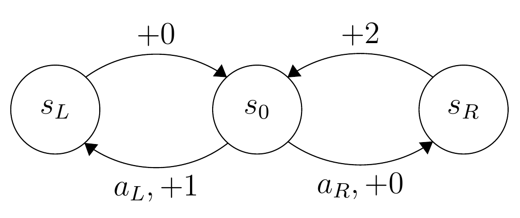
The edges represent the state transitions given an action, as well as the reward received. For example, in state $s_0$, taking action $a_L$ means the new state is $s_L$, and the reward received is $+1$. The transitions leading out from $s_L$ and $s_R$ are independant of action. This gives us effectively two choices of deterministic policies, $\pi_L(s_0) = s_L$ and $\pi_R(s_0) = s_R$ (it is irrelevant what those policies do in the other states.)
Your task here is to compute the value $V_{\pi}(s_0)$ for $\pi = \pi_L$ and $\pi = \pi_R$. Which policy is better? Does the answer depend on the choice of discount factor $\gamma$? If so, how?
Answer
Following the first policy, this gives
Tabular RL, Known Environments
For the moment, we focus on environments for which the agent has access to $T$ and $R$, which will allow us to solve the Bellman equation explicitly.
We will also assume that the policy $\pi$ is a deterministic mapping from state to action, and denote $a_t = \pi(s_t)$. This means we can drop the sum $\sum_a$ in the Bellman equation, and write:
and in $Q$-value form:
Below, we've provided a simple environment for a gridworld taken from Russell and Norvig. The agent can choose one of four actions: up (0), right (1), down (2) and left (3), encoded as numbers. The observation is just the state that the agent is in (states are labelled left-to-right, top-to-bottom, from 0 to 11).
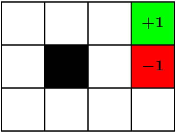
The result of choosing an action will move the agent in that direction, unless they would bump into a wall $\fcolorbox{grey}{grey}{\phantom{-1}}$ or walk outside the grid, in which case the agent doesn't move. Both the $\fcolorbox{lightgreen}{lightgreen}{\textcolor{black}{+1}}$ (heaven) and $\fcolorbox{red}{red}{\textcolor{black}{-1}}$ (hell) terminal states "trap" the agent, and any movement from one of the terminal states leaves the agent in the same state, and no reward is received. The agent receives a small penalty for each move $r = -0.04$ to encourage them to move to a terminal state quickly, unless the agent is moving into a terminal state, in which case they receive reward either $+1$ or $-1$ as appropriate.
Lastly, the environment is slippery, and the agent only has a 70\% chance of moving in the direction chosen, with a 10% chance each of attempting to move in the other three cardinal directions.
From the bottom right cell, there are two possible routes to heaven: A short path that goes past hell, and the path that goes the long way around the wall. Which one do you think the agent will prefer? How do you think changing the penalty value r=-0.04 to something else might affect this?
The long route requires more steps, which (assuming $r<0$) will be penalised more, but due to the 30\% probability of slipping, walking near the $\fcolorbox{red}{red}{\textcolor{black}{-1}}$ means the agent might fall into it by mistake, so the agent should avoid getting anywhere close to it.
We can guess that there is a certain threshold value $r^*$ such that the optimal policy follows the short route for harsher penalty $r
You can test this out (and find the approximate value of $r^*$) when you run your RL agent!
Provided is a class that allows us to define environments with known dynamics. The only parts you should be concerned with are
.num_states : int, which gives the number of states,.num_actions : int, which gives the number of actions.T : Float[Tensor, "num_states num_actions num_states"]which represents the transitional probability $T(s_{\text{new}} \mid s, a)$ =T[s, a, s_new].R : Float[Tensor, "num_states num_actions num_states"]which represents the reward function $R(s,a,s_{\text{new}})$ =R[s,a,s_new]associated with entering state $s_{\text{new}}$ from state $s$ by taking action $a$.
This environment also provides two additional parameters which we will not use now, but needed later where the environment is treated as a black box, and agents learn from interaction.
* .start, the state with which interaction with the environment begins. By default, assumed to be state zero.
* .terminal, a list of all the terminal states (with which interaction with the environment ends). By default, assumed that there are no terminal states.
class Environment:
    def __init__(self, num_states: int, num_actions: int, start=0, terminal=None):
        self.num_states = num_states
        self.num_actions = num_actions
        self.start = start
        self.terminal = np.array([], dtype=int) if terminal is None else terminal
        (self.T, self.R) = self.build()

    def build(self):
        """
        Constructs the T and R tensors from the dynamics of the environment.

        Returns:
            T : (num_states, num_actions, num_states) State transition probabilities
            R : (num_states, num_actions, num_states) Reward function
        """
        num_states = self.num_states
        num_actions = self.num_actions
        T = np.zeros((num_states, num_actions, num_states))
        R = np.zeros((num_states, num_actions, num_states))
        for s in range(num_states):
            for a in range(num_actions):
                (states, rewards, probs) = self.dynamics(s, a)
                (all_s, all_r, all_p) = self.out_pad(states, rewards, probs)
                T[s, a, all_s] = all_p
                R[s, a, all_s] = all_r
        return (T, R)

    def dynamics(self, state: int, action: int) -> tuple[Arr, Arr, Arr]:
        """
        Computes the distribution over possible outcomes for a given state
        and action.

        Args:
            state  : int (index of state)
            action : int (index of action)

        Returns:
            states  : (m,) all the possible next states
            rewards : (m,) rewards for each next state transition
            probs   : (m,) likelihood of each state-reward pair
        """
        raise NotImplementedError()

    def render(pi: Arr):
        """
        Takes a policy pi, and draws an image of the behavior of that policy, if applicable.

        Args:
            pi : (num_actions,) a policy

        Returns:
            None
        """
        raise NotImplementedError()

    def out_pad(self, states: Arr, rewards: Arr, probs: Arr):
        """
        Args:
            states  : (m,) all the possible next states
            rewards : (m,) rewards for each next state transition
            probs   : (m,) likelihood of each state-reward pair

        Returns:
            states  : (num_states,) all the next states
            rewards : (num_states,) rewards for each next state transition
            probs   : (num_states,) likelihood of each state-reward pair (including zero-prob outcomes.)
        """
        out_s = np.arange(self.num_states)
        out_r = np.zeros(self.num_states)
        out_p = np.zeros(self.num_states)
        for i in range(len(states)):
            idx = states[i]
            out_r[idx] += rewards[i]
            out_p[idx] += probs[i]
        return out_s, out_r, out_p
For example, here is the toy environment from the theory exercises earlier (the 3-state environment) implemented in this format.
Note - don't spend too much time reading this code and the plots generated below; this is just designed to illustrate how we can implement a particular environment on top of our class above by defining certain environment dynamics. The environment you'll actually be working with is the gridworld environment described above.
class Toy(Environment):
    def dynamics(self, state: int, action: int):
        """
        Sets up dynamics for the toy environment:
            - In state s_L, we move to s_0 & get +0 reward regardless of action
            - In state s_R, we move to s_0 & get +2 reward regardless of action
            - In state s_0,
                - action LEFT=0 leads to s_L & get +1,
                - action RIGHT=1 leads to s_R & get +0
        """
        (SL, S0, SR) = (0, 1, 2)
        LEFT = 0

        assert 0 <= state < self.num_states and 0 <= action < self.num_actions

        if state == S0:
            (next_state, reward) = (SL, 1) if action == LEFT else (SR, 0)
        elif state == SL:
            (next_state, reward) = (S0, 0)
        elif state == SR:
            (next_state, reward) = (S0, 2)
        else:
            raise ValueError(f"Invalid state: {state}")

        return (np.array([next_state]), np.array([reward]), np.array([1]))

    def __init__(self):
        super().__init__(num_states=3, num_actions=2)
Given a definition for the dynamics function, the Environment class automatically generates T and R for us. We can plot these below:
- The first plot shows transition probabilities $T(s_{next} \mid s, a)$. It has only probabilities of 1 and 0 because transitions are deterministic ($s_{next}$ is a function of $s$ and $a$). At $s_L$ or $s_R$ you'll move back to the center $s_0$ regardless of what action you take, but at $s_0$ you can move either left or right and it will have different outcomes.
- The second plot shows rewards $R(s, a, s_{next})$. The rewards are $1$ for $s_0 \to s_L$, and $2$ for $s_R \to s_0$, and zero reward for all other possible transitions.
Note that the environment being deterministic means the reward is uniquely determined by $s$ and $a$ (because $s_{next}$ is a function of $s$ and $a$). This won't always be the case in RL, as we move to more complex environments.
toy = Toy()

actions = ["a_L", "a_R"]
states = ["s_L", "s_0", "s_R"]

imshow(
    toy.T,  # dimensions (s, a, s_next)
    title="Transition probabilities T(s_next | s, a) for toy environment",
    facet_col=0,
    facet_labels=[f"Current state is s = {s}" for s in states],
    y=actions,
    x=states,
    labels={
        "x": "Next state, s_next",
        "y": "Action taken, a",
        "color": "Transition<br>Probability",
    },
    text_auto=".0f",
    border=True,
    width=850,
    height=350,
)

imshow(
    toy.R,  # dimensions (s, a, s_next)
    title="Rewards R(s, a, s_next) for toy environment",
    facet_col=0,
    facet_labels=[f"Current state is s = {s}" for s in states],
    y=actions,
    x=states,
    labels={"x": "Next state, s_next", "y": "Action taken, a", "color": "Reward"},
    text_auto=".0f",
    border=True,
    width=850,
    height=350,
)
Click to see the expected output
We also provide an implementation of the gridworld environment above.
The dynamics function sets up the dynamics of the Gridworld environment: if the agent takes an action, there is a 70% chance the action is successful, and 10% chance the agent moves in one of the other 3 directions randomly. The rest of the code here deals with edge cases like hitting a wall or being in a terminal state. It's not important to fully read through & understand how this method works.
We include a definition of render, which given a policy, prints out a grid showing the direction the policy will try to move in from each cell.
class Norvig(Environment):
    def dynamics(self, state: int, action: int) -> tuple[Arr, Arr, Arr]:
        def state_index(state):
            assert 0 <= state[0] < self.width and 0 <= state[1] < self.height, print(state)
            pos = state[0] + state[1] * self.width
            assert 0 <= pos < self.num_states, print(state, pos)
            return pos

        pos = self.states[state]
        if state in self.terminal or state in self.walls:
            return (np.array([state]), np.array([0]), np.array([1]))
        out_probs = np.zeros(self.num_actions) + 0.1
        out_probs[action] = 0.7
        out_states = np.zeros(self.num_actions, dtype=int) + self.num_actions
        out_rewards = np.zeros(self.num_actions) + self.penalty
        new_states = [pos + x for x in self.actions]
        for i, s_new in enumerate(new_states):
            if not (0 <= s_new[0] < self.width and 0 <= s_new[1] < self.height):
                out_states[i] = state
                continue
            new_state = state_index(s_new)
            if new_state in self.walls:
                out_states[i] = state
            else:
                out_states[i] = new_state
            for idx in range(len(self.terminal)):
                if new_state == self.terminal[idx]:
                    out_rewards[i] = self.goal_rewards[idx]
        return (out_states, out_rewards, out_probs)

    def render(self, pi: Arr):
        assert len(pi) == self.num_states
        emoji = ["⬆️", "➡️", "⬇️", "⬅️"]
        grid = [emoji[act] for act in pi]
        grid[3] = "🟩"
        grid[7] = "🟥"
        grid[5] = "⬛"
        print("".join(grid[0:4]) + "\n" + "".join(grid[4:8]) + "\n" + "".join(grid[8:]))

    def __init__(self, penalty=-0.04):
        self.height = 3
        self.width = 4
        self.penalty = penalty
        num_states = self.height * self.width
        num_actions = 4
        self.states = np.array([[x, y] for y in range(self.height) for x in range(self.width)])
        self.actions = np.array([[0, -1], [1, 0], [0, 1], [-1, 0]])
        self.dim = (self.height, self.width)
        terminal = np.array([3, 7], dtype=int)
        self.walls = np.array([5], dtype=int)
        self.goal_rewards = np.array([1.0, -1])
        super().__init__(num_states, num_actions, start=8, terminal=terminal)


# Example use of `render`: print out a random policy
norvig = Norvig()
pi_random = np.random.randint(0, 4, (12,))
norvig.render(pi_random)
Policy Evaluation
At the moment, we would like to determine the value function $V_\pi$ of some policy $\pi$. We will assume policies are deterministic, and encode policies as a lookup table from states to actions (so $\pi$ will be a vector of length num_states, and $\pi(i)$ is the action we take at state $i$).
Firstly, we will use the Bellman equation as an update rule: Given a current estimate $\hat{V}_\pi$ of the value function $V_{\pi}$, we can obtain a better estimate by using the Bellman equation, sweeping over all states.
Why does iterating the Bellman equation converge to the correct answer?
We proved above in a drop-down that the Bellman equation is a contraction mapping, and so the iteration converges to the (unique) fixed point, and the fixed point is the exact value function, as we proved that it satisfies the Bellman equation.
Exercise - implement policy_eval_numerical
The policy_eval_numerical function takes in a deterministic policy $\pi$ and transition & reward matrices $T$ and $R$, and computes the value function $V_\pi$ using the Bellman equation as an update rule. It keeps iterating, computing estimates $\hat{V}^1_\pi, \hat{V}^2_\pi, \ldots$ until it reaches max_iterations, or we terminate after $n$ iterations, where
$n$ is the first value for which $|| \hat{V}_\pi^{n+1} - \hat{V}_\pi^n ||_\infty < \epsilon$ - which ever comes first.
Recall - we store our transition and reward matrices as env.T and env.R, where we define env.T[s, a, s'] $= T(s' \,|\, s, a)$ and env.R[s, a, s'] $= R(s, a, s')$.
def policy_eval_numerical(env: Environment, pi: Arr, gamma=0.99, eps=1e-8, max_iterations=10_000) -> Arr:
    """
    Numerically evaluates the value of a given policy by iterating the Bellman equation
    Args:
        env: Environment
        pi : shape (num_states,) - The policy to evaluate
        gamma: float - Discount factor
        eps  : float - Tolerance
        max_iterations: int - Maximum number of iterations to run
    Outputs:
        value : float (num_states,) - The value function for policy pi
    """
    num_states = env.num_states

    raise NotImplementedError()


tests.test_policy_eval(policy_eval_numerical, exact=False)
Help - I'm stuck on the iterative formula
You can start by indexing env.T[range(num_states), pi, :], which effectively gives you the transition matrix with shape (num_states, num_states) with values $T(s' \,|\, s, \pi(s))$ for all $s, s'$ (since the action $\pi(s)$ is a deterministic function of the starting state $s$). You can do exactly the same for env.R to get the reward matrix.
If you prefer, you can also write this using Callum's eindex notation:
T_pi = eindex(env.T, pi, "s [s] s_new -> s s_new")
Next, you can apply the update formula by multiplying these tensors and summing over $s'$. Be careful of tensor shapes and broadcasting!
Solution
def policy_eval_numerical(env: Environment, pi: Arr, gamma=0.99, eps=1e-8, max_iterations=10_000) -> Arr:
    """
    Numerically evaluates the value of a given policy by iterating the Bellman equation
    Args:
        env: Environment
        pi : shape (num_states,) - The policy to evaluate
        gamma: float - Discount factor
        eps  : float - Tolerance
        max_iterations: int - Maximum number of iterations to run
    Outputs:
        value : float (num_states,) - The value function for policy pi
    """
    num_states = env.num_states

    value = np.zeros((num_states,))
    transition_matrix = env.T[range(num_states), pi, :]  # shape [s, s_next]
    reward_matrix = env.R[range(num_states), pi, :]  # shape [s, s_next]

    for i in range(max_iterations):
        new_value = einops.reduce(transition_matrix * (reward_matrix + gamma * value), "s s_next -> s", "sum")

        delta = np.abs(new_value - value).max()
        if delta < eps:
            break
        value = np.copy(new_value)
    else:
        print(f"Failed to converge after {max_iterations} steps.")

    return value
Exact Policy Evaluation
Essentially what we are doing in the previous step is solving the Bellman equation via iteration. However, we can actually solve it directly in this case, since it's effectively just a set of linear equations! In future cases we won't be able to because we won't know all the transition probabilities & rewards, but here we can solve directly.
To do this, let's define the transition matrix $\mathbf{P}^\pi$ and reward matrix $\mathbf{R}^\pi$ just like we did in the solution to the previous exercise:
Intuition for this equation
One nice intuition comes from the Taylor expansion $(\mathbf{I} - \mathbf{X})^{-1} = \mathbf{I} + \mathbf{X} + \mathbf{X}^2 + \ldots$ which is valid for any matrix $\mathbf{X}$ with $||\mathbf{X}|| < 1$. Applying this to our equation, we get:
Exercise - implement policy_eval_exact
The function below should apply the exact policy evaluation formula to solve for $\mathbf{v}^\pi$ directly.
You can start by defining the same transition_matrix and reward_matrix as in the previous exercise. You may also find the function np.linalg.solve helpful: given matrix equation $\mathbf{A} \mathbf{x} = \mathbf{b}$, then np.linalg.solve(A,b) returns x, assuming a solution exists.
def policy_eval_exact(env: Environment, pi: Arr, gamma=0.99) -> Arr:
    """
    Finds the exact solution to the Bellman equation.
    """
    num_states = env.num_states

    raise NotImplementedError()


tests.test_policy_eval(policy_eval_exact, exact=True)
Solution
def policy_eval_exact(env: Environment, pi: Arr, gamma=0.99) -> Arr:
    """
    Finds the exact solution to the Bellman equation.
    """
    num_states = env.num_states

    transition_matrix = env.T[range(num_states), pi, :]  # shape [s, s_next]
    reward_matrix = env.R[range(num_states), pi, :]  # shape [s, s_next]

    r = einops.einsum(transition_matrix, reward_matrix, "s s_next, s s_next -> s")

    mat = np.eye(num_states) - gamma * transition_matrix

    return np.linalg.solve(mat, r)
Policy Improvement
Now we can evaluate a policy, we want to improve it. One way we can do this is to compare how well $\pi$ performs on a state versus the value obtained by choosing another action instead, that is, the Q-value. If there is an action $a'$ for which $Q_{\pi}(s,a') > V_\pi(s) \equiv Q_\pi(s, \pi(s))$, then action $a'$ is preferable over action $\pi(s)$ in state $s$. Recall that we could write out our Bellman equation like this:
which gives us an update rule for our policy $\pi$, given that we've evaluated $V_\pi$ using our closed-form expression from earlier, by choosing a better action according to what maximises the RHS of the Bellman equation. Or in other words:
Exercise - implement policy_improvement
The policy_improvement function takes in a value function $V$, and transition and reward tensors $T$ and $R$, and returns a new policy $\pi^\text{better}$.
Recall, we've defined our objects as env.T[s, a, s'] $= T(s' \,|\, a, s)$, and env.R[s, a, s'] $= R(s, a, s')$.
def policy_improvement(env: Environment, V: Arr, gamma=0.99) -> Arr:
    """
    Args:
        env: Environment
        V  : (num_states,) value of each state following some policy pi
    Outputs:
        pi_better : vector (num_states,) of actions representing a new policy obtained via policy
                    iteration
    """
    raise NotImplementedError()


tests.test_policy_improvement(policy_improvement)
Solution
def policy_improvement(env: Environment, V: Arr, gamma=0.99) -> Arr:
    """
    Args:
        env: Environment
        V  : (num_states,) value of each state following some policy pi
    Outputs:
        pi_better : vector (num_states,) of actions representing a new policy obtained via policy
                    iteration
    """
    q_values_for_every_state_action_pair = einops.einsum(env.T, env.R + gamma * V, "s a s_next, s a s_next -> s a")
    pi_better = q_values_for_every_state_action_pair.argmax(axis=1)
    return pi_better
Note, the reason our solution works is that computing env.R + gamma & V correctly broadcasts V: it has dimensions (s_next,), and env.R has dimensions (s, a, s_next).
Putting these together, we now have an algorithm to find the optimal policy for an environment.
We alternate policy evaluation ($\overset{E}{\to}$) and policy improvement ($\overset{I}{\to}$), with each improvement step being a strict monotonic improvement,
Exercise - implement find_optimal_policy
Implement the find_optimal_policy function below. This should iteratively do the following:
- find the correct value function $V_{\pi}$ for your given policy $\pi$ using your
policy_eval_exactfunction, - update your policy using
policy_improvement,
The first policy $\pi_0$ is arbitrary (we've picked all zeros).
A few things to note:
- Don't forget that policies should be of
dtype=int, rather than floats! $\pi$ in this case represents the deterministic action you take in each state. - Since optimal policies may not be unique, the automated tests will merely check that your optimal policy has the same value function as the optimal policy found by the solution.
def find_optimal_policy(env: Environment, gamma=0.99, max_iterations=10_000):
    """
    Args:
        env: environment
    Outputs:
        pi : (num_states,) int, of actions represeting an optimal policy
    """
    pi = np.zeros(shape=env.num_states, dtype=int)

    raise NotImplementedError()


tests.test_find_optimal_policy(find_optimal_policy)

penalty = -1
norvig = Norvig(penalty)
pi_opt = find_optimal_policy(norvig, gamma=0.99)
norvig.render(pi_opt)
Solution
def find_optimal_policy(env: Environment, gamma=0.99, max_iterations=10_000):
    """
    Args:
        env: environment
    Outputs:
        pi : (num_states,) int, of actions represeting an optimal policy
    """
    pi = np.zeros(shape=env.num_states, dtype=int)

    for i in range(max_iterations):
        V = policy_eval_exact(env, pi, gamma)
        pi_new = policy_improvement(env, V, gamma)
        if np.array_equal(pi_new, pi):
            return pi_new
        else:
            pi = pi_new
    else:
        print(f"Failed to converge after {max_iterations} steps.")
        return pi
Once you've passed the tests, you should play around with the penalty value for the gridworld environment and see how this affects the optimal policy found. Which squares change their optimal strategy when the penalty takes different negative values (e.g. -0.04, -0.1, or even -1). To see why this happens, refer back to the dropdown earlier, in the section "Tabular RL, Known Environments". Can you see why the different rewards lead to the behaviours that they do?
Bonus
- Implement and test your policy evaluation method on other environments.
- Complete some exercises in Chapters 3 and 4 of Sutton and Barto.
- Modify the tabular RL solvers to allow stochastic policies or to allow $\gamma=1$ on episodic environments (may need to change how environments are defined.)