5️⃣ Sparse Autoencoders in Toy Models

Learning Objectives

• Learn about sparse autoencoders, and how they might be used to disentangle features represented in superposition
• Train your own SAEs on the toy models from earlier sections, and visualise the feature reconstruction process
• Understand important SAE training strategies (e.g. resampling) and architecture variants (e.g. Gated, Jump ReLU)

We now move on to sparse autoencoders, a recent line of work that has been explored by Anthropic in their recent paper, and is currently one of the most interesting areas of research in mechanistic interpretability.

In the following set of exercises, you will:

• Build your own sparse autoencoder, writing its architecture & loss function,
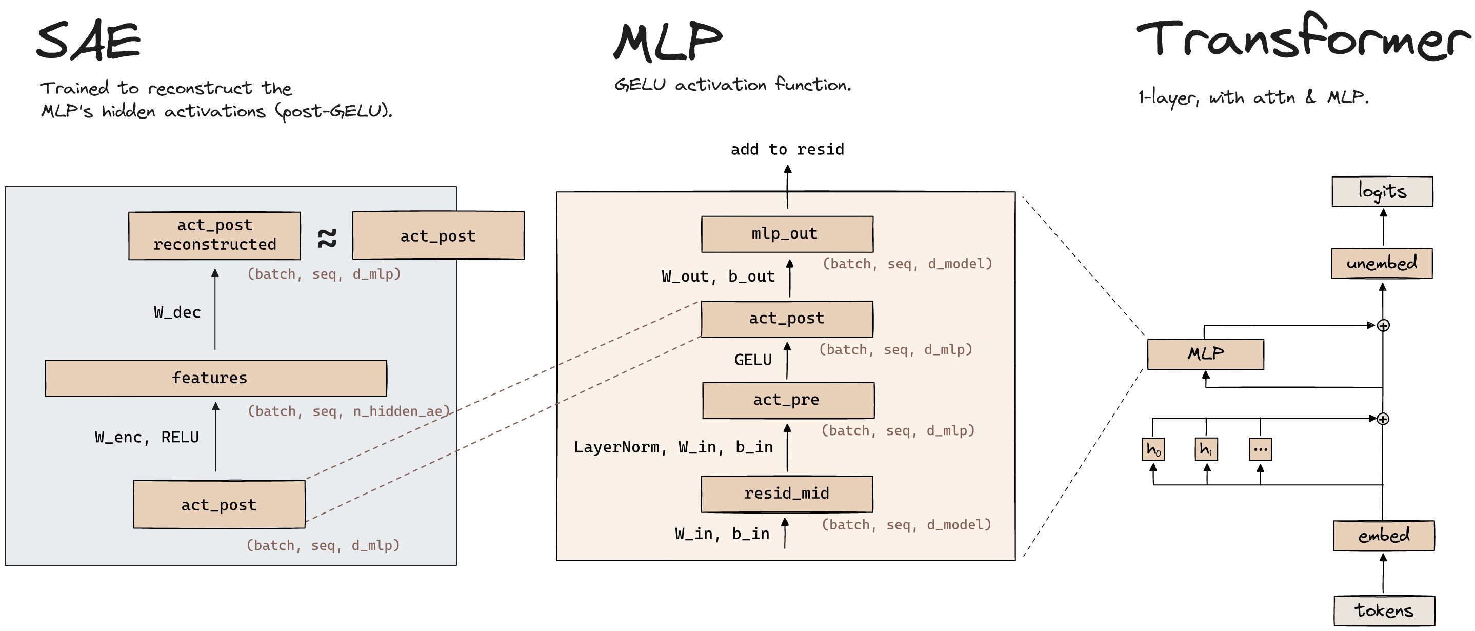
• Train your SAE on the hidden activations of the Model class which you defined earlier (note the difference between this and the Anthropic paper's setup, since the latter trained SAEs on the MLP layer, whereas we're training it on a non-privileged basis),
• Extract the features from your SAE, and verify that these are the same as your model's learned features.

You should read Anthropic's dictionary learning paper (linked above): the introduction and first section (problem setup) up to and including the "Sparse Autoencoder Setup" section. Make sure you can answer at least the following questions:

What is an autoencoder, and what is it trained to do?

Autoencoders are a type of neural network which learns efficient encodings / representations of unlabelled data. It is trained to compress the input in some way to a latent representation, then map it back into the original input space. It is trained by minimizing the reconstruction loss between the input and the reconstructed input.

The "encoding" part usually refers to the latent space being lower-dimensional than the input. However, that's not always the case, as we'll see with sparse autoencoders.

Why does the L1 penalty encourage sparsity? (This isn't specifically mentioned in this paper, but it's an important thing to understand.)

Unlike $L_2$ penalties, the $L_1$ penalty actually pushes values towards zero. This is a well-known result in statistics, best illustrated below:

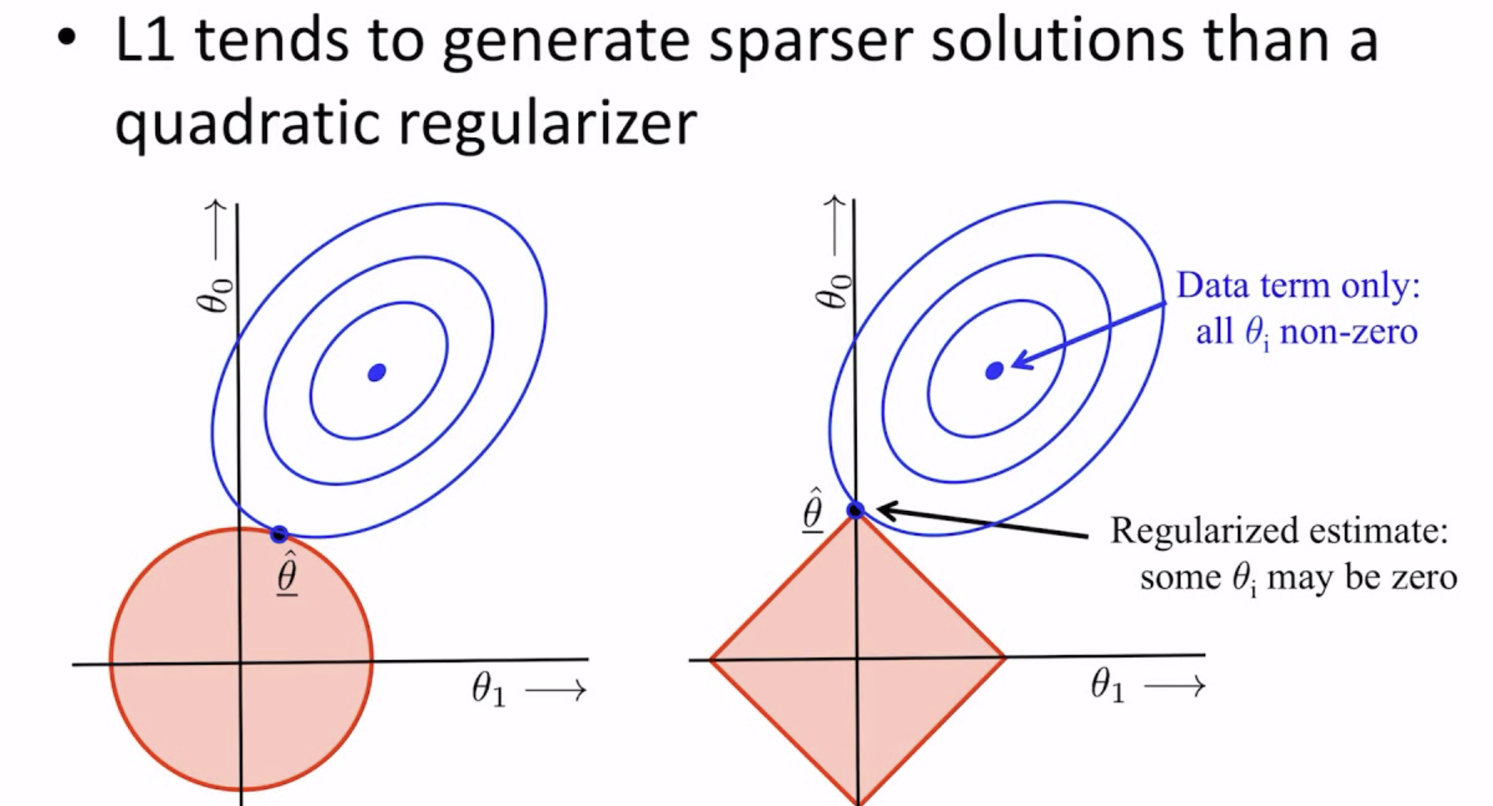
See [this Google ML page](https://developers.google.com/machine-learning/crash-course/regularization-for-sparsity/l1-regularization) for more of an explanation (it also has a nice out-of-context animation!).

Problem setup

Recall the setup of our previous model:

We're going to train our autoencoder to just take in the hidden state activations $h$, map them to a larger (overcomplete) hidden state $z$, then reconstruct the original hidden state $h$ from $z$.

Note the choice to have a different encoder and decoder weight matrix, rather than having them tied - we'll discuss this more later.

It's important not to get confused between the autoencoder and model's notation. Remember - the model takes in features $x$, maps them to lower-dimensional vectors $h$, and then reconstructs them as $x'$. The autoencoder takes in these hidden states $h$, maps them to a higher-dimensional but sparse vector $z$, and then reconstructs them as $h'$. Our hope is that the elements of $z$ correspond to the features of $x$.

Another note - the use of $b_{dec}$ here might seem weird, since we're subtracting it at the start then adding it back at the end. The way we're treating this term is as a centralizing term for the hidden states. It subtracts some learned mean vector from them so that $W_{enc}$ can act on centralized vectors, and then this term gets added back to the reconstructed hidden states at the end of the model.

Notation

The autoencoder's hidden activations go by many names. Sometimes they're called neurons (since they do have an activation function applied to them which makes them a privileged basis, like the neurons in an MLP layer). Sometimes they're called features, since the idea with SAEs is that these hidden activations are meant to refer to specific features in the data. However, the word feature is a bit overloaded - ideally we want to use "feature" to refer to the attributes of the data itself - if our SAE's weights are randomly initialized, is it fair to call this a feature?!

For this reason, we'll be referring to the autoencoder's hidden activations as SAE latents. However, it's worth noting that people sometimes use "SAE features" or "neurons" instead, so try not to get confused (e.g. often people use "neuron resampling" to refer to the resampling of the weights in the SAE).

The new notation we'll adopt in this section is:

• d_sae, which is the number of activations in the SAE's hidden layer (i.e. the latent dimension). Note that we want the SAE latents to correspond to the original data features, which is why we'll need d_sae >= n_features (usually we'll have equality in this section).
• d_in, which is the SAE input dimension. This is the same as d_hidden from the previous sections because the SAE is reconstructing the model's hidden activations, however calling it d_hidden in the context of an SAE would be confusing. Usually in this section, we'll have d_in = d_hidden = 2, so we can visualize the results.

SAE class

We've provided the ToySAEConfig class below. Its arguments are as follows (we omit the ones you'll only need to work with in later exercises):

• n_inst, which means the same as it does in your ToyModel class
• d_in, the input size to your SAE (equal to d_hidden of your ToyModel class)
• d_sae, the SAE's latent dimension size
• sparsity_coeff, which is used in your loss function
• weight_normalize_eps, which is added to the denominator whenever you normalize weights
• tied_weights, which is a boolean determining whether your encoder and decoder weights are tied
• ste_epsilon, which is only relevant for JumpReLU SAEs later on

We've also given you the ToySAE class. Your job over the next 4 exercises will be to fill in the __init__, W_dec_normalized, generate_batch and forward methods.

@dataclass
class ToySAEConfig:
    n_inst: int
    d_in: int
    d_sae: int
    sparsity_coeff: float = 0.2
    weight_normalize_eps: float = 1e-8
    tied_weights: bool = False
    ste_epsilon: float = 0.01


class ToySAE(nn.Module):
    W_enc: Float[Tensor, "inst d_in d_sae"]
    _W_dec: Float[Tensor, "inst d_sae d_in"] | None
    b_enc: Float[Tensor, "inst d_sae"]
    b_dec: Float[Tensor, "inst d_in"]

    def __init__(self, cfg: ToySAEConfig, model: ToyModel) -> None:
        super(ToySAE, self).__init__()

        assert cfg.d_in == model.cfg.d_hidden, "Model's hidden dim doesn't match SAE input dim"
        self.cfg = cfg
        self.model = model.requires_grad_(False)
        self.model.W.data[1:] = self.model.W.data[0]
        self.model.b_final.data[1:] = self.model.b_final.data[0]

        raise NotImplementedError()

        self.to(device)

    @property
    def W_dec(self) -> Float[Tensor, "inst d_sae d_in"]:
        return self._W_dec if self._W_dec is not None else self.W_enc.transpose(-1, -2)

    @property
    def W_dec_normalized(self) -> Float[Tensor, "inst d_sae d_in"]:
        """
        Returns decoder weights, normalized over the autoencoder input dimension.
        """
        # You'll fill this in later
        raise NotImplementedError()

    def generate_batch(self, batch_size: int) -> Float[Tensor, "batch inst d_in"]:
        """
        Generates a batch of hidden activations from our model.
        """
        # You'll fill this in later
        raise NotImplementedError()

    def forward(
        self, h: Float[Tensor, "batch inst d_in"]
    ) -> tuple[
        dict[str, Float[Tensor, "batch inst"]],
        Float[Tensor, "batch inst"],
        Float[Tensor, "batch inst d_sae"],
        Float[Tensor, "batch inst d_in"],
    ]:
        """
        Forward pass on the autoencoder.

        Args:
            h: hidden layer activations of model

        Returns:
            loss_dict:       dict of different loss terms, each having shape (batch_size, n_inst)
            loss:            total loss (i.e. sum over terms of loss dict), same shape as loss terms
            acts_post:       autoencoder latent activations, after applying ReLU
            h_reconstructed: reconstructed autoencoder input
        """
        # You'll fill this in later
        raise NotImplementedError()

    def optimize(
        self,
        batch_size: int = 1024,
        steps: int = 10_000,
        log_freq: int = 100,
        lr: float = 1e-3,
        lr_scale: Callable[[int, int], float] = constant_lr,
        resample_method: Literal["simple", "advanced", None] = None,
        resample_freq: int = 2500,
        resample_window: int = 500,
        resample_scale: float = 0.5,
        hidden_sample_size: int = 256,
    ) -> list[dict[str, Any]]:
        """
        Optimizes the autoencoder using the given hyperparameters.

        Args:
            model:              we reconstruct features from model's hidden activations
            batch_size:         size of batches we pass through model & train autoencoder on
            steps:              number of optimization steps
            log_freq:           number of optimization steps between logging
            lr:                 learning rate
            lr_scale:           learning rate scaling function
            resample_method:    method for resampling dead latents
            resample_freq:      number of optimization steps between resampling dead latents
            resample_window:    number of steps needed for us to classify a neuron as dead
            resample_scale:     scale factor for resampled neurons
            hidden_sample_size: size of hidden value sample we add to the logs (for visualization)

        Returns:
            data_log:           dictionary containing data we'll use for visualization
        """
        assert resample_window <= resample_freq

        optimizer = t.optim.Adam(self.parameters(), lr=lr)  # betas=(0.0, 0.999)
        frac_active_list = []
        progress_bar = tqdm(range(steps))

        # Create lists of dicts to store data we'll eventually be plotting
        data_log = []

        for step in progress_bar:
            # Resample dead latents
            if (resample_method is not None) and ((step + 1) % resample_freq == 0):
                frac_active_in_window = t.stack(frac_active_list[-resample_window:], dim=0)
                if resample_method == "simple":
                    self.resample_simple(frac_active_in_window, resample_scale)
                elif resample_method == "advanced":
                    self.resample_advanced(frac_active_in_window, resample_scale, batch_size)

            # Update learning rate
            step_lr = lr * lr_scale(step, steps)
            for group in optimizer.param_groups:
                group["lr"] = step_lr

            # Get a batch of hidden activations from the model
            with t.inference_mode():
                h = self.generate_batch(batch_size)

            # Optimize
            loss_dict, loss, acts, _ = self.forward(h)
            loss.mean(0).sum().backward()
            optimizer.step()
            optimizer.zero_grad()

            # Normalize decoder weights by modifying them directly (if not using tied weights)
            if not self.cfg.tied_weights:
                self.W_dec.data = self.W_dec_normalized.data

            # Calculate the mean sparsities over batch dim for each feature
            frac_active = (acts.abs() > 1e-8).float().mean(0)
            frac_active_list.append(frac_active)

            # Display progress bar, and log a bunch of values for creating plots / animations
            if step % log_freq == 0 or (step + 1 == steps):
                progress_bar.set_postfix(
                    lr=step_lr,
                    loss=loss.mean(0).sum().item(),
                    frac_active=frac_active.mean().item(),
                    **{k: v.mean(0).sum().item() for k, v in loss_dict.items()},  # type: ignore
                )
                with t.inference_mode():
                    loss_dict, loss, acts, h_r = self.forward(
                        h := self.generate_batch(hidden_sample_size)
                    )
                data_log.append(
                    {
                        "steps": step,
                        "frac_active": (acts.abs() > 1e-8).float().mean(0).detach().cpu(),
                        "loss": loss.detach().cpu(),
                        "h": h.detach().cpu(),
                        "h_r": h_r.detach().cpu(),
                        **{name: param.detach().cpu() for name, param in self.named_parameters()},
                        **{name: loss_term.detach().cpu() for name, loss_term in loss_dict.items()},
                    }
                )

        return data_log

    @t.no_grad()
    def resample_simple(
        self,
        frac_active_in_window: Float[Tensor, "window inst d_sae"],
        resample_scale: float,
    ) -> None:
        """
        Resamples dead latents, by modifying the model's weights and biases inplace.

        Resampling method is:
            - For each dead neuron, generate a random vector of size (d_in,), and normalize these vecs
            - Set new values of W_dec and W_enc to be these normalized vecs, at each dead neuron
            - Set b_enc to be zero, at each dead neuron
        """
        raise NotImplementedError()

    @t.no_grad()
    def resample_advanced(
        self,
        frac_active_in_window: Float[Tensor, "window inst d_sae"],
        resample_scale: float,
        batch_size: int,
    ) -> None:
        """
        Resamples latents that have been dead for `dead_feature_window` steps, according to `frac_active`.

        Resampling method is:
            - Compute the L2 reconstruction loss produced from the hidden state vecs `h`
            - Randomly choose values of `h` with probability proportional to their reconstruction loss
            - Set new values of W_dec & W_enc to be these centered & normalized vecs, at each dead neuron
            - Set b_enc to be zero, at each dead neuron
        """
        raise NotImplementedError()

Exercise - implement __init__

You should implement the __init__ method below. This should define the weights b_enc, b_dec, W_enc and _W_dec. Use Kaiming uniform for weight initialization, and initialize the biases at zero.

Note, we use _W_dec to handle the case of tied weights: it should be None if we have tied weights, and a proper parameter if we don't have tied weights. The property W_dec we've given you in the class above will deal with both cases for you.

Why might we want / not want to tie our weights?

In our Model implementations, we used a weight and its transpose. You might think it also makes sense to have the encoder and decoder weights be transposed copies of each other, since intuitively both the encoder and decoder's latent vectors meant to represent some feature's "direction in the original model's hidden dimension".

The reason we might not want to tie weights is pretty subtle. The job of the encoder is in some sense to recover features from superposition, whereas the job of the decoder is just to represent that feature faithfully if present (since the goal of our SAE is to write the input as a linear combination of W_dec vectors) - this is why we generally see the decoder weights as the "true direction" for a feature, when weights are untied.

The diagram below might help illustrate this concept (if you want, you can replicate the results in this diagram using our toy model setup!).

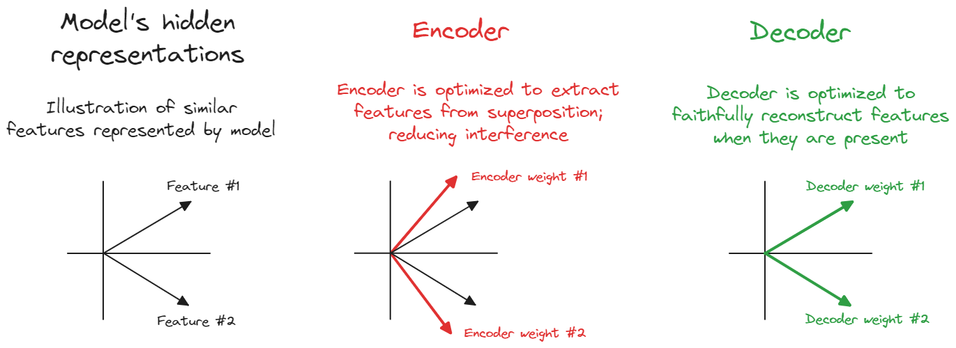
In simple settings like this toy model we might not benefit much from untying weights, and tying weights can actually help us avoid finding annoying local minima in our optimization. However, for most of these exercises we'll use untied weights in order to illustrate SAE concepts more clearly.

Also, note that we've defined self.cfg and self.model for you in the init function - in the latter case, we've frozen the model's weights (because when you train your SAE you don't want to track gradients in your base model), and we've also modified the model's weights so they all match the first instance (this is so we can more easily interpret our SAE plots we'll create when we finish training).

# Go back up and edit your `ToySAE.__init__` method, then run the test below

tests.test_sae_init(ToySAE)

def __init__(self: ToySAE, cfg: ToySAEConfig, model: ToyModel) -> None:
    super(ToySAE, self).__init__()
assert cfg.d_in == model.cfg.d_hidden, "Model's hidden dim doesn't match SAE input dim"
    self.cfg = cfg
    self.model = model.requires_grad_(False)
    self.model.W.data[1:] = self.model.W.data[0]
    self.model.b_final.data[1:] = self.model.b_final.data[0]
self.W_enc = nn.Parameter(nn.init.kaiming_uniform_(t.empty((cfg.n_inst, cfg.d_in, cfg.d_sae))))
    self._W_dec = (
        None
        if self.cfg.tied_weights
        else nn.Parameter(nn.init.kaiming_uniform_(t.empty((cfg.n_inst, cfg.d_sae, cfg.d_in))))
    )
    self.b_enc = nn.Parameter(t.zeros(cfg.n_inst, cfg.d_sae))
    self.b_dec = nn.Parameter(t.zeros(cfg.n_inst, cfg.d_in))
self.to(device)
ToySAE.__init__ = __init__

Exercise - implement W_dec_normalized

You should now fill in the W_dec_normalized property, which returns the decoder weights, normalized (with L2 norm) over the autoencoder input dimension. Note that the existence of the W_dec property means you can safety refer to this attribute, without having to worry about _W_dec any more. Also, remember to add cfg.weight_normalize_eps to your denominator (this helps avoid divide-by-zero errors).

# Go back up and edit your `ToySAE.W_dec_normalized` method, then run the test below

tests.test_sae_W_dec_normalized(ToySAE)

@property
def W_dec_normalized(self: ToySAE) -> Float[Tensor, "inst d_sae d_in"]:
    """Returns decoder weights, normalized over the autoencoder input dimension."""
    return self.W_dec / (self.W_dec.norm(dim=-1, keepdim=True) + self.cfg.weight_normalize_eps)
ToySAE.W_dec_normalized = W_dec_normalized

Exercise - implement generate_batch

As mentioned, our data no longer comes directly from ToyModel.generate_batch. Instead, we use Model.generate_batch to get our model input $x$, and then apply our model's W matrix to get its hidden activations $h=Wx$. Note that we're working with the model from the "Superposition in a Nonprivileged Basis" model, meaning there's no ReLU function to apply to get $h$.

You should fill in the generate_batch method now, then run the test. Note - remember to use self.model rather than model!

# Go back up and edit your `ToySAE.generate_batch` method, then run the test below

tests.test_sae_generate_batch(ToySAE)

def generate_batch(self: ToySAE, batch_size: int) -> Float[Tensor, "batch inst d_in"]:
    """
    Generates a batch of hidden activations from our model.
    """
    return einops.einsum(
        self.model.generate_batch(batch_size),
        self.model.W,
        "batch inst feats, inst d_in feats -> batch inst d_in",
    )
ToySAE.generate_batch = generate_batch

Exercise - implement forward

You should calculate the autoencoder's hidden state activations as $z = \operatorname{ReLU}(W_{enc}(h - b_{dec}) + b_{enc})$, and then reconstruct the output as $h' = W_{dec}z + b_{dec}$. A few notes:

• The first variable we return is a loss_dict, which contains the loss tensors of shape (batch_size, n_inst) for both terms in our loss function (before multiplying by the L1 coefficient). This is used for logging, and it'll also be used later in our neuron resampling methods. For this architecture, your keys should be "L_reconstruction" and "L_sparsity".
• The second variable we return is the loss term, which also has shape (batch_size, n_inst), and is created by summing the losses in loss_dict (with sparsity loss multiplied by cfg.sparsity_coeff). When doing gradient descent, we'll average over the batch dimension & sum over the instance dimension (since we're training our instances independently & in parallel).
• The third variable we return is the hidden state activations acts, which are also used later for neuron resampling (as well as logging how many latents are active).
• The fourth variable we return is the reconstructed hidden states h_reconstructed, i.e. the autoencoder's actual output.

An important note regarding our loss term - the reconstruction loss is the squared difference between input & output averaged over the d_in dimension, but the sparsity penalty is the L1 norm of the hidden activations summed over the d_sae dimension. Can you see why we average one but sum the other?

Note - make sure you're using self.W_dec_normalized rather than self.W_dec in your forward function. This is because if we're using tied weights then we won't be able to manually normalize W_dec inplace, but we still want to use the normalized version.

# Go back up and edit your `ToySAE.forward` method, then run the test below

tests.test_sae_forward(ToySAE)

def forward(
    self: ToySAE, h: Float[Tensor, "batch inst d_in"]
) -> tuple[
    dict[str, Float[Tensor, "batch inst"]],
    Float[Tensor, "batch inst"],
    Float[Tensor, "batch inst d_sae"],
    Float[Tensor, "batch inst d_in"],
]:
    """
    Forward pass on the autoencoder.
    Args:
        h: hidden layer activations of model
    Returns:
        loss_dict:       dict of different loss terms, each dict value having shape (batch_size, n_inst)
        loss:            total loss (i.e. sum over terms of loss dict), same shape as loss_dict values
        acts_post:       autoencoder latent activations, after applying ReLU
        h_reconstructed: reconstructed autoencoder input
    """
    h_cent = h - self.b_dec
# Compute latent (hidden layer) activations
    acts_pre = (
        einops.einsum(h_cent, self.W_enc, "batch inst d_in, inst d_in d_sae -> batch inst d_sae")
        + self.b_enc
    )
    acts_post = F.relu(acts_pre)
# Compute reconstructed input
    h_reconstructed = (
        einops.einsum(
            acts_post, self.W_dec_normalized, "batch inst d_sae, inst d_sae d_in -> batch inst d_in"
        )
        + self.b_dec
    )
# Compute loss terms
    L_reconstruction = (h_reconstructed - h).pow(2).mean(-1)
    L_sparsity = acts_post.abs().sum(-1)
    loss_dict = {"L_reconstruction": L_reconstruction, "L_sparsity": L_sparsity}
    loss = L_reconstruction + self.cfg.sparsity_coeff * L_sparsity
return loss_dict, loss, acts_post, h_reconstructed
ToySAE.forward = forward

Training your SAE

The optimize method has been given to you. A few notes on how it differs from your previous model:

• Before each optimization step, we implement neuron resampling - we'll get to this later.
• We have more logging, via the data_log dictionary - we'll use this for visualization.
• We've used betas=(0.0, 0.999), to match the description in Anthropic's Feb 2024 update - although they document it to work better specifically for large models, we may as well match it here.

First, let's define and train our model, and visualize model weights and the data returned from sae.generate_batch (which are the hidden state representations of our trained model, and will be used for training our SAE).

Note that we'll use a feature probability of 2.5% (and assume independence between features) for all subsequent exercises.

d_hidden = d_in = 2
n_features = d_sae = 5
n_inst = 16

# Create a toy model, and train it to convergence
cfg = ToyModelConfig(n_inst=n_inst, n_features=n_features, d_hidden=d_hidden)
model = ToyModel(cfg=cfg, device=device, feature_probability=0.025)
model.optimize()

sae = ToySAE(cfg=ToySAEConfig(n_inst=n_inst, d_in=d_in, d_sae=d_sae), model=model)

h = sae.generate_batch(512)

utils.plot_features_in_2d(model.W[:8], title="Base model")
utils.plot_features_in_2d(
    einops.rearrange(h[:, :8], "batch inst d_in -> inst d_in batch"),
    title="Hidden state representation of a random batch of data",
)

Now, let's train our SAE, and visualize the instances with lowest loss! We've also created a function animate_features_in_2d which creates an animation of the training over time. If the inline displaying doesn't work, you might have to open the saved HTML file in your browser to see it.

data_log = sae.optimize(steps=20_000)

utils.animate_features_in_2d(
    data_log,
    instances=list(range(8)),  # only plot the first 8 instances
    rows=["W_enc", "_W_dec"],
    filename=str(section_dir / "animation-training.html"),
    title="SAE on toy model",
)

# If this display code doesn't work, try saving & opening animation in your browser
with open(section_dir / "animation-training.html") as f:
    display(HTML(f.read()))

In other words, the autoencoder is generally successful at reconstructing the model's hidden states, and maybe sometimes it learns the fully monosemantic solution (one latent per feature), but more often it learns a combination of polysemantic latents and dead latents (which never activate). These are a big problem because they don't receive any gradients during training, so they're not a problem which fixes itself over time. You can check the presence of dead latents by graphing the feature probabilities over training, in the code below. You should find that:

1. Some latents are dead for most or all of training (with "fraction of datapoints active" being zero),
2. Some latents fire more frequently than the target feature prob of 2.5% (these are usually polysemantic, i.e. they fire on more than one different feature),
3. Some latents fire approximately at or slightly below the target probability (these are usually monosemantic). If any of your instances above learned the full monosemantic solution (i.e. latents uniformly spaced around the 2D hidden dimension) then you should find that all 5 latents in that instance fall into this third category.

utils.frac_active_line_plot(
    frac_active=t.stack([data["frac_active"] for data in data_log]),
    title="Probability of sae features being active during training",
    avg_window=20,
)

Resampling

From Anthropic's paper (replacing terminology "dead neurons" with "dead latents" in accordance with how we're using the term):

Second, we found that over the course of training some latents cease to activate, even across a large number of datapoints. We found that “resampling” these dead latents during training gave better results by allowing the model to represent more features for a given autoencoder hidden layer dimension. Our resampling procedure is detailed in Autoencoder Resampling, but in brief we periodically check for latents which have not fired in a significant number of steps and reset the encoder weights on the dead latents to match data points that the autoencoder does not currently represent well.

Your next task is to implement this resampling procedure.

Exercise - implement resample_simple

The process Anthropic describes for resampling SAE latents is pretty involved, so we'll start by implementing a simpler version of it. Specifically, we'll implement the following algorithm for each instance inst:

• Find all the dead latents (i.e. the values (inst, d) where frac_active_in_window[:, inst, d] are all zero).
• For each of these, do the following:
  • Generate a new random vector v of length d_in.
  • Set the decoder weights W_dec[inst, d, :] to this new vector v, normalized.
  • Set the encoder weights W_enc[inst, :, d] to this new vector v, scaled to have norm resample_scale.
  • Set the encoder biases b_enc[inst, d] to zero.

The test function we've given you will check that your function replaces / zeros the correct weights.

# Go back up and edit your `ToySAE.resample_simple` method, then run the test below

tests.test_resample_simple(ToySAE)

@t.no_grad()
def resample_simple(
    self: ToySAE,
    frac_active_in_window: Float[Tensor, "window inst d_sae"],
    resample_scale: float,
) -> None:
    """
    Resamples dead latents, by modifying the model's weights and biases inplace.
    Resampling method is:
        - For each dead neuron, generate a random vector of size (d_in,), and normalize these vecs
        - Set new values of W_dec and W_enc to be these normalized vectors, at each dead neuron
        - Set b_enc to be zero, at each dead neuron
    This function performs resampling over all instances at once, using batched operations.
    """
    # Get a tensor of dead latents
    dead_latents_mask = (frac_active_in_window < 1e-8).all(dim=0)  # [instances d_sae]
    n_dead = int(dead_latents_mask.int().sum().item())
# Get our random replacement values of shape [n_dead d_in], and scale them
    replacement_values = t.randn((n_dead, self.cfg.d_in), device=self.W_enc.device)
    replacement_values_normed = replacement_values / (
        replacement_values.norm(dim=-1, keepdim=True) + self.cfg.weight_normalize_eps
    )
# Change the corresponding values in W_enc, W_dec, and b_enc
    self.W_enc.data.transpose(-1, -2)[dead_latents_mask] = (
        resample_scale * replacement_values_normed
    )
    self.W_dec.data[dead_latents_mask] = replacement_values_normed
    self.b_enc.data[dead_latents_mask] = 0.0
ToySAE.resample_simple = resample_simple

Once you've passed the tests, train your model again, and watch the animation to see how the neuron resampling has helped the training process. You should be able to see the resampled neurons in red.

resampling_sae = ToySAE(cfg=ToySAEConfig(n_inst=n_inst, d_in=d_in, d_sae=d_sae), model=model)

resampling_data_log = resampling_sae.optimize(steps=20_000, resample_method="simple")

utils.animate_features_in_2d(
    resampling_data_log,
    rows=["W_enc", "_W_dec"],
    instances=list(range(8)),  # only plot the first 8 instances
    filename=str(section_dir / "animation-training-resampling.html"),
    color_resampled_latents=True,
    title="SAE on toy model (with resampling)",
)

utils.frac_active_line_plot(
    frac_active=t.stack([data["frac_active"] for data in resampling_data_log]),
    title="Probability of sae features being active during training",
    avg_window=20,
)

Much better!

Now that we have pretty much full reconstruction on our features, let's visualize that reconstruction! The animate_features_in_2d function also offers features to plot hidden state reconstructions and how they evolve over time. Examining how the hidden state reconstructions evolve over time can help you understand what's going on, for example:

• The SAE often learns a non-sparse solution (e.g. 4 uniformly spaced polysemantic latents & 1 dead latent) before converging to the ideal solution.
  • Note, we also see something similar when training SAEs on LLMs: they first find a non-sparse solution with small reconstruction loss, before learning a more sparse solution (L0 goes down).
• Hovering over hidden states, you should observe some things:
  • Low-magnitude hidden states are often reconstructed as zero, this is because the SAE can't separate them from interference from other features.
  • Even for correctly reconstructed features, the hidden state magnitude is generally smaller than the true hidden states - this is called shrinkage, and we'll discuss it extensively in the next section.

utils.animate_features_in_2d(
    resampling_data_log,
    rows=["W_enc", "h", "h_r"],
    instances=list(range(4)),  # plotting fewer instances for a smaller animation file size
    color_resampled_latents=True,
    filename=str(section_dir / "animation-training-reconstructions.html"),
    title="SAE on toy model (showing hidden states & reconstructions)",
)

Exercise - implement resample_advanced

This section can be considered optional if you've already implemented the simpler version of resample above. However, if you're interested in a version of it which hues close to Anthropic's methodology, then you might still be interested in this exercise.

The main difference we'll make is in how the resampled values are chosen. Rather than just drawing them randomly from a distribution and normalizing them, we'll be sampling them with replacement from a set of input activations $h$, with sampling probabilities weighted by the squared $L_2$ loss of the autoencoder on each input. Intuitively, this will make it more likely that our resampled neurons will represent feature directions that the autoencoder is currently doing a bad job of representing.

The new resampling algorithm looks like the following - for each instance we:

• Generate a batch of hidden data h from your SAE and compute its squared reconstruction loss l2_squared. It should have shape (batch_size, n_inst). If the L2 loss for this instance l2_squared[:, inst] is zero everywhere, we can skip this instance.
• Find the dead latents for this instance (i.e. the instances inst and latent indices d where frac_active_in_window[:, inst, d] are all zero).
• For each of these, do the following:
  • Randomly sample a vector v = h[x, inst, :], where 0 <= x < batch_size is chosen according to the distribution with probabilities proportional to l2_squared[:, inst].
  • Set the decoder weights W_dec[inst, d, :] to this new vector v, normalized.
  • Set the encoder weights W_enc[inst, :, d] to this new vector v, scaled to have norm resample_scale * avg_W_enc_alive_norm (where the term avg_W_enc_alive_norm is the mean norm of the encoder weights of alive neurons for that particular instance).
  • Set the encoder biases b_enc[inst, d] to zero.

So we really have just 2 changes: the added use of avg_W_enc_alive_norm for the encoder weights, and the sampling from the L2-based distribution to get our vectors v. Because this function can get a bit messy, we recommend you iterate through the instances rather than trying to resample them all at once.

For the sampling, we recommend that you use torch.distributions.categorical.Categorical to define a probability distribution, which can then be sampled from using the sample method. We've included an example of how to use this function below.

from torch.distributions.categorical import Categorical
# Define a prob distn over (0, 1, 2, 3, 4) with probs proportional to (4, 3, 2, 1, 0)
values = t.arange(5).flip(0)
probs = values.float() / values.sum()
distribution = Categorical(probs = probs)
# Sample a single value from it
distribution.sample() # tensor(1)
# Sample multiple values with replacement (values will mostly be in the lower end of the range)
distribution.sample((10,)) # tensor([1, 1, 3, 0, 0, 1, 0, 3, 2, 2])

Once you've implemented this resampling method, run the tests:

# Go back up and edit your `ToySAE.resample_advanced` method, then run the test below

tests.test_resample_advanced(ToySAE)

@t.no_grad()
def resample_advanced(
    self: ToySAE,
    frac_active_in_window: Float[Tensor, "window inst d_sae"],
    resample_scale: float,
    batch_size: int,
) -> None:
    """
    Resamples latents that have been dead for 'dead_feature_window' steps, according to frac_active.
    Resampling method is:
        - Compute the L2 reconstruction loss produced from the hidden state vectors h
        - Randomly choose values of h with probability proportional to their reconstruction loss
        - Set new values of W_dec & W_enc to be these centered & normalized vecs, at each dead neuron
        - Set b_enc to be zero, at each dead neuron
    Returns colors and titles (useful for creating the animation: resampled neurons appear in red).
    """
    h = self.generate_batch(batch_size)
    l2_loss = self.forward(h)[0]["L_reconstruction"]
for instance in range(self.cfg.n_inst):
        # Find the dead latents in this instance. If all latents are alive, continue
        is_dead = (frac_active_in_window[:, instance] < 1e-8).all(dim=0)
        dead_latents = t.nonzero(is_dead).squeeze(-1)
        n_dead = dead_latents.numel()
        if n_dead == 0:
            continue  # If we have no dead features, then we don't need to resample
# Compute L2 loss for each element in the batch
        l2_loss_instance = l2_loss[:, instance]  # [batch_size]
        if l2_loss_instance.max() < 1e-6:
            continue  # If we have zero reconstruction loss, we don't need to resample
# Draw d_sae samples from [0, 1, ..., batch_size-1], with probabilities proportional to
        # the values of l2_loss
        distn = Categorical(probs=l2_loss_instance.pow(2) / l2_loss_instance.pow(2).sum())
        replacement_indices = distn.sample((n_dead,))  # type: ignore
# Index into the batch of hidden activations to get our replacement values
        replacement_values = (h - self.b_dec)[replacement_indices, instance]  # [n_dead d_in]
        replacement_values_normalized = replacement_values / (
            replacement_values.norm(dim=-1, keepdim=True) + self.cfg.weight_normalize_eps
        )
# Get the norm of alive neurons (or 1.0 if there are no alive neurons)
        W_enc_norm_alive_mean = (
            self.W_enc[instance, :, ~is_dead].norm(dim=0).mean().item() if (~is_dead).any() else 1.0
        )
# Lastly, set the new weights & biases (W_dec is normalized, W_enc needs specific scaling,
        # b_enc is zero)
        self.W_dec.data[instance, dead_latents, :] = replacement_values_normalized
        self.W_enc.data[instance, :, dead_latents] = (
            replacement_values_normalized.T  W_enc_norm_alive_mean  resample_scale
        )
        self.b_enc.data[instance, dead_latents] = 0.0
ToySAE.resample_advanced = resample_advanced

After passing the tests, you can try training & visualizing your SAE again. You might not spot a lot of improvement with this resampling method in 2 dimensions, but for much higher-dimensional spaces it becomes highly beneficial to resample neurons in a more targeted way.

Gated & JumpReLU SAEs

In these sections, we'll discuss two alternative SAE architectures that seem to offer performance improvement over standard models. Both of them have similar intuitions (and are actually close to being mathematically equivalent under certain assumptions), although we'll focus on Gated SAEs first before moving to JumpReLU. This isn't necessarily because they're conceptually simpler (there's an argument that JumpReLU is simpler), it's more because they're easier to train. However, it's worth remembering during this section that both architectures are important and effective, and the intuitions from one often carry over to the other.

Gated SAEs

There are many different SAE architecture variants being explored at the moment. One especially exciting one is the Gated SAE, described in detail in this paper from DeepMind. We can motivate this architecture by starting with two observations

1. Empirically, features usually seem to want to be binary. For instance, we often see features like "is this about a basketball" which are better thought of as "off" or "on" than occupying some continuous range from 0 to 1. In practice reconstructing the precise coefficients does matter, and they often seem important for indicating something like the model's confidence in a particular feature being present. But still, we'd ideally like an architecture which can learn this discontinuity.

One easy option would be to have a discontinuous activation function in the hidden layer of our SAE, such as a Jump ReLU. This activation has a jump at some value $\theta$, and could allow us to represent this nonlinearity.

However, there's another problem which Jump ReLUs alone** won't solve:

1. SAEs suffer from shrinkage. Recall that the actual objective we want is that the L0 "norm" (the number of non-zero elements) of the hidden layer is small, and we use the L1 norm as a proxy for this. The two loss term in the SAE loss function have conflicting goals: the reconstruction term wants to make the autoencoder good at reconstructing the input, and the sparsity term wants to shrink the magnitude of the hidden layer. This means that even when perfect reconstruction is possible with only a single hidden unit activated, the sparsity loss will bias the magnitude of this hidden unit to zero, and the reconstruction will be worse.

**Note, JumpReLUs alone don't fix shrinkage, but JumpReLUs plus L0 penalty does fix shrinkage - we'll discuss this later in the chapter.

This brings us to Gated SAEs, which seem to fix both problems by having a Heaviside term which applies a discontinuity, and decoupling this term from the magnitude term. Instead of our standard function for computing SAE activations:

we instead use:

You might be wondering, how can we train this SAE? Ideally we'd place a sparsity penalty on the term $f_{\text{gate}}(\mathbf{x})$, since that's the thing which determines whether our activations will be zero or not. Unfortunately we can't do that, because gradients won't propagate through the Heaviside function (it's discontinuous). Instead, we apply a sparsity penalty to the preactivation $\pi_{\text {gate }}(\mathbf{x})$. So we have our loss function:

However, there's a problem here. As long as the preactivation values $\pi_{\text {gate }}(\mathbf{x})$ are positive, reducing them will reduce the sparsity penalty without changing the reconstruction loss (all that matters for reconstruction is whether the preactivation values are positive or negative). So eventually they'll hit zero, and won't receive any more gradients (because the model's output will just always be zero from that point onwards). To combat this, we add an auxiliary loss term equal to the reconstruction loss when we swap out the true latent activations for the preactivation values $\pi_{\text {gate }}(\mathbf{x})$. This will add a gradient for the preactivations which pushes them up, offsetting the sparsity loss function which will only push those values down towards zero. We now have our final loss function:

Exercise - implement Gated SAEs

Now, you have all the information you need to implement a Gated SAE and compare it to the standard model. Below we've given you the GatedToySAE class which should have modified versions of the ToySAE methods, in accordance with the descriptions above.

Note - an alternative way of implementing this would be to modify your ToySAE class to support both gated and standard architectures, e.g. by introducing an architecture argument in your SAE config class. You're encouraged to try this as a bonus exercise if you think it would be good practice for you!

Some tips:

• For the forward pass and the loss function, you can reference Appendix G in the DeepMind paper, on page 34. We recommend sticking to the naming convention used by that appendix, as you'll probably find this easiest.
• Remember to create and resample different weights if you're using the Gated architecture. For instance, if Gated then you should be zeroing b_mag, b_gate and r_mag at all dead latents.
• We recommend you tie the gate and magnitude weights by default, i.e. as $\left(\mathbf{W}_{\text {mag }}\right)_{i j}:=\exp \left(\mathbf{r}_{\text {mag }}\right)_i \times \left(\mathbf{W}_{\text {gate }}\right)_{i j}$ like they do in the paper. This kind of tying is arguably a lot less unnatural than tying encoder & decoder weights. If you're also tying weights, then you can interpret that as $W_{\text{dec}} = W_{\text{gate}}$.

@property
def W_mag(self) -> Float[Tensor, "inst d_in d_sae"]:
    assert self.cfg.architecture == "gated", "W_mag only available for gated model"
    return self.r_mag.exp().unsqueeze(1) * self.W_gate

class GatedToySAE(ToySAE):
    W_gate: Float[Tensor, "inst d_in d_sae"]
    b_gate: Float[Tensor, "inst d_sae"]
    r_mag: Float[Tensor, "inst d_sae"]
    b_mag: Float[Tensor, "inst d_sae"]
    _W_dec: Float[Tensor, "inst d_sae d_in"] | None
    b_dec: Float[Tensor, "inst d_in"]

    def __init__(self, cfg: ToySAEConfig, model: ToyModel):
        super(ToySAE, self).__init__()

        # YOUR CODE HERE - initialize the Gated model's weights & biases
        raise NotImplementedError()

        self.to(device)

    @property
    def W_dec(self) -> Float[Tensor, "inst d_sae d_in"]:
        # YOUR CODE HERE - return the decoder weights. Depending on what you name your
        # weights in __init__, this may not differ from the `ToySAE` implementation.
        raise NotImplementedError()

    @property
    def W_mag(self) -> Float[Tensor, "inst d_in d_sae"]:
        # YOUR CODE HERE - implement the magnitude weights getter (tied as described above).
        raise NotImplementedError()

    def forward(
        self, h: Float[Tensor, "batch inst d_in"]
    ) -> tuple[
        dict[str, Float[Tensor, "batch inst"]],
        Float[Tensor, ""],
        Float[Tensor, "batch inst d_sae"],
        Float[Tensor, "batch inst d_in"],
    ]:
        """
        Same as previous forward function, but allows for gated case as well (in which case we have
        different functional form, as well as a new term "L_aux" in the loss dict).
        """
        # YOUR CODE HERE - implement the Gated forward function. This will be similar
        # to the standard forward function, but with the gating mechanism included
        # (plus a new loss term "L_aux" in the loss dict).
        raise NotImplementedError()

        assert sorted(loss_dict.keys()) == ["L_aux", "L_reconstruction", "L_sparsity"]
        return loss_dict, loss, acts_post, h_reconstructed

    @t.no_grad()
    def resample_simple(
        self, frac_active_in_window: Float[Tensor, "window inst d_sae"], resample_scale: float
    ) -> None:
        # YOUR CODE HERE - implement the resample_simple function for the Gated SAE.
        # This will be identical to the ToySAE implementation, except that it will
        # apply to different weights & biases.
        raise NotImplementedError()

    @t.no_grad()
    def resample_advanced(
        self,
        frac_active_in_window: Float[Tensor, "window inst d_sae"],
        resample_scale: float,
        batch_size: int,
    ) -> None:
        # YOUR CODE HERE - implement the resample_advanced function for the Gated SAE.
        # This will be identical to the ToySAE implementation, except that it will
        # apply to different weights & biases.
        raise NotImplementedError()

class GatedToySAE(ToySAE):
    W_gate: Float[Tensor, "inst d_in d_sae"]
    b_gate: Float[Tensor, "inst d_sae"]
    r_mag: Float[Tensor, "inst d_sae"]
    b_mag: Float[Tensor, "inst d_sae"]
    _W_dec: Float[Tensor, "inst d_sae d_in"] | None
    b_dec: Float[Tensor, "inst d_in"]
def __init__(self, cfg: ToySAEConfig, model: ToyModel):
        super(ToySAE, self).__init__()
assert cfg.d_in == model.cfg.d_hidden, "ToyModel's hidden dim doesn't match SAE input dim"
        self.cfg = cfg
        self.model = model.requires_grad_(False)
        self.model.W.data[1:] = self.model.W.data[0]
        self.model.b_final.data[1:] = self.model.b_final.data[0]
self._W_dec = (
            None
            if self.cfg.tied_weights
            else nn.Parameter(nn.init.kaiming_uniform_(t.empty((cfg.n_inst, cfg.d_sae, cfg.d_in))))
        )
        self.b_dec = nn.Parameter(t.zeros(cfg.n_inst, cfg.d_in))
self.W_gate = nn.Parameter(
            nn.init.kaiming_uniform_(t.empty((cfg.n_inst, cfg.d_in, cfg.d_sae)))
        )
        self.b_gate = nn.Parameter(t.zeros(cfg.n_inst, cfg.d_sae))
        self.r_mag = nn.Parameter(t.zeros(cfg.n_inst, cfg.d_sae))
        self.b_mag = nn.Parameter(t.zeros(cfg.n_inst, cfg.d_sae))
self.to(device)
@property
    def W_dec(self) -> Float[Tensor, "inst d_sae d_in"]:
        return self._W_dec if self._W_dec is not None else self.W_gate.transpose(-1, -2)
@property
    def W_mag(self) -> Float[Tensor, "inst d_in d_sae"]:
        return self.r_mag.exp().unsqueeze(1)  self.W_gate
def forward(
        self, h: Float[Tensor, "batch inst d_in"]
    ) -> tuple[
        dict[str, Float[Tensor, "batch inst"]],
        Float[Tensor, ""],
        Float[Tensor, "batch inst d_sae"],
        Float[Tensor, "batch inst d_in"],
    ]:
        """
        Same as previous forward function, but allows for gated case as well (in which case we have
        different functional form, as well as a new term "L_aux" in the loss dict).
        """
        h_cent = h - self.b_dec
# Compute the gating terms (pi_gate(x) and f_gate(x) in the paper)
        gating_pre_activation = (
            einops.einsum(
                h_cent, self.W_gate, "batch inst d_in, inst d_in d_sae -> batch inst d_sae"
            )
            + self.b_gate
        )
        active_features = (gating_pre_activation > 0).float()
# Compute the magnitude term (f_mag(x) in the paper)
        magnitude_pre_activation = (
            einops.einsum(
                h_cent, self.W_mag, "batch inst d_in, inst d_in d_sae -> batch inst d_sae"
            )
            + self.b_mag
        )
        feature_magnitudes = F.relu(magnitude_pre_activation)
# Compute the hidden activations (f˜(x) in the paper)
        acts_post = active_features  feature_magnitudes
# Compute reconstructed input
        h_reconstructed = (
            einops.einsum(
                acts_post, self.W_dec, "batch inst d_sae, inst d_sae d_in -> batch inst d_in"
            )
            + self.b_dec
        )
# Compute loss terms
        gating_post_activation = F.relu(gating_pre_activation)
        via_gate_reconstruction = (
            einops.einsum(
                gating_post_activation,
                self.W_dec.detach(),
                "batch inst d_sae, inst d_sae d_in -> batch inst d_in",
            )
            + self.b_dec.detach()
        )
        loss_dict = {
            "L_reconstruction": (h_reconstructed - h).pow(2).mean(-1),
            "L_sparsity": gating_post_activation.sum(-1),
            "L_aux": (via_gate_reconstruction - h).pow(2).sum(-1),
        }
loss = (
            loss_dict["L_reconstruction"]
            + self.cfg.sparsity_coeff  loss_dict["L_sparsity"]
            + loss_dict["L_aux"]
        )
assert sorted(loss_dict.keys()) == ["L_aux", "L_reconstruction", "L_sparsity"]
        return loss_dict, loss, acts_post, h_reconstructed
@t.no_grad()
    def resample_simple(
        self, frac_active_in_window: Float[Tensor, "window inst d_sae"], resample_scale: float
    ) -> None:
        dead_latents_mask = (frac_active_in_window < 1e-8).all(dim=0)  # [instances d_sae]
        n_dead = int(dead_latents_mask.int().sum().item())
replacement_values = t.randn((n_dead, self.cfg.d_in), device=self.W_gate.device)
        replacement_values_normed = replacement_values / (
            replacement_values.norm(dim=-1, keepdim=True) + self.cfg.weight_normalize_eps
        )
# New names for weights & biases to resample
        self.W_gate.data.transpose(-1, -2)[dead_latents_mask] = (
            resample_scale  replacement_values_normed
        )
        self.W_dec.data[dead_latents_mask] = replacement_values_normed
        self.b_mag.data[dead_latents_mask] = 0.0
        self.b_gate.data[dead_latents_mask] = 0.0
        self.r_mag.data[dead_latents_mask] = 0.0
@t.no_grad()
    def resample_advanced(
        self,
        frac_active_in_window: Float[Tensor, "window inst d_sae"],
        resample_scale: float,
        batch_size: int,
    ) -> None:
        h = self.generate_batch(batch_size)
        l2_loss = self.forward(h)[0]["L_reconstruction"]
for instance in range(self.cfg.n_inst):
            is_dead = (frac_active_in_window[:, instance] < 1e-8).all(dim=0)
            dead_latents = t.nonzero(is_dead).squeeze(-1)
            n_dead = dead_latents.numel()
            if n_dead == 0:
                continue
l2_loss_instance = l2_loss[:, instance]  # [batch_size]
            if l2_loss_instance.max() < 1e-6:
                continue
distn = Categorical(probs=l2_loss_instance.pow(2) / l2_loss_instance.pow(2).sum())
            replacement_indices = distn.sample((n_dead,))  # type: ignore
replacement_values = (h - self.b_dec)[replacement_indices, instance]  # [n_dead d_in]
            replacement_values_normalized = replacement_values / (
                replacement_values.norm(dim=-1, keepdim=True) + self.cfg.weight_normalize_eps
            )
W_gate_norm_alive_mean = (
                self.W_gate[instance, :, ~is_dead].norm(dim=0).mean().item()
                if (~is_dead).any()
                else 1.0
            )
# New names for weights & biases to resample
            self.W_dec.data[instance, dead_latents, :] = replacement_values_normalized
            self.W_gate.data[instance, :, dead_latents] = (
                replacement_values_normalized.T  W_gate_norm_alive_mean  resample_scale
            )
            self.b_mag.data[instance, dead_latents] = 0.0
            self.b_gate.data[instance, dead_latents] = 0.0
            self.r_mag.data[instance, dead_latents] = 0.0

Now, you can run the code below to train a Gated SAE and visualize the results. Note that we're only plotting the best 4/16 instances (ranked according to loss averaged over the last 10 sampled batches), since generally SAEs with thresholding on toy models tend to more easily collapse into local minima (I suspect this is because thresholding flattens the loss landscape and allows more exploration & finding of local minima, whereas simple SAE architectures are more directly funnelled towards the global minimum).

gated_sae = GatedToySAE(
    cfg=ToySAEConfig(
        n_inst=n_inst,
        d_in=d_in,
        d_sae=d_sae,
        sparsity_coeff=1.0,
    ),
    model=model,
)
gated_data_log = gated_sae.optimize(steps=20_000, resample_method="advanced")

# Animate the best instances, ranked according to average loss near the end of training
n_inst_to_plot = 4
n_batches_for_eval = 10
avg_loss = t.concat([d["loss"] for d in gated_data_log[-n_batches_for_eval:]]).mean(0)
best_instances = avg_loss.topk(n_inst_to_plot, largest=False).indices.tolist()

utils.animate_features_in_2d(
    gated_data_log,
    rows=["W_gate", "_W_dec", "h", "h_r"],
    instances=best_instances,
    filename=str(section_dir / "animation-training-gated.html"),
    color_resampled_latents=True,
    title="SAE on toy model",
)

Exercise - demonstrate advantage of Gated models

When thinking about how thresholding models like Gated & JumpReLU can outperform standard SAEs, the plot to have in your head is the one below, from the appendix of DeepMind's Gated SAEs paper. The left histogram shows the distribution along a particular feature direction - the blue represents the distribution from interference when the feature is off but other non-orthogonal features are on, and the red represents the distribution then the feature is on. The distributions form a clearly bimodal pattern, and we can see in the figure on the right how a jump discontinuity (like the one provided by ReLU or by Gated models) can better model this discontinuity, by correctly reconstructing more of the interference cases (blue) as zero.

Although our data distribution isn't exactly the same as the one here, it is still bimodal: the histogram of "projection along feature direction $f$ conditional on $f$ being active" will have a significantly greater mean than the histogram of "projection along feature direction $f$ conditional on $f$ being inactive". In fact, you can try replicating this exact plot yourself and showing exactly how your Gated model outperforms the standard model.

We've left this exercise relatively open-ended rather than just being a function to fill in. If you want to attempt it, we recommend you get help from Claude or ChatGPT to create the visualization - the important part is understanding the plot well enough to know what data you need to gather in order to replicate it. Also, note that our toy model setup is slightly different from the paper's - we're using 5 independent features and so the "X off" distribution is down to interference from the other features, whereas the paper only considers a single feature and predefines an "X on" and "X off" distribution. The docstring should help you better understand what plot we're making here.

If you want, you can also extend the function generate_batch so that it supports a normal distribution with most of its probability mass in the range [0, 1] (this is what the feat_mag_distn field in the ToyModelConfig class is for) so that it more closely matches the distribution in the paper's toy model setup. However, you shouldn't have to do this to replicate the key result.

YOUR CODE HERE - replicate figure 15a & 15b from the paper

def generate_batch(self: ToyModel, batch_size: int) -> Float[Tensor, "batch inst feats"]:
    """
    Generates a batch of data of shape (batch_size, n_instances, n_features).
    This is optional, we just provide the function for you here to use for completeness (the code
    run below will not use "normal" distribution mode to generate the data), it'll use the same
    "unif" mode we've used so far.)
    """
    assert self.cfg.feat_mag_distn in ["unif", "normal"], (
        f"Unknown feature distribution: {self.cfg.feat_mag_distn}"
    )
batch_shape = (batch_size, self.cfg.n_inst, self.cfg.n_features)
    feat_seeds = t.rand(batch_shape, device=self.W.device)
    feat_mag = (
        t.rand(batch_shape, device=self.W.device)
        if self.cfg.feat_mag_distn == "unif"
        else t.clip(0.5 + 0.2  t.randn(batch_shape, device=self.W.device), min=0.0, max=1.0)
    )
    return t.where(feat_seeds <= self.feature_probability, feat_mag, 0.0)
ToyModel.generate_batch = generate_batch
@t.inference_mode()
def replicate_figure_15(sae_tuples: list[tuple[str, ToySAE, list[dict[str, Any]]]]) -> None:
    """
    This function should replicate figure 15 from the DeepMind paper, in a way which conforms to our
    toy model setup. It should create 2 plots:
        (1) A histogram of activation distributions projected along some chosen feature direction,
            color coded according to whether that feature is active or inactive. You should find
            that the distribution when active is almost always positive, and the distribution when
            not active has mean below zero.
        (2) A scatter plot of SAE reconstructions. In other words, the x-axis values should be the
            original feature values, and the y-axis should be the SAE's reconstructions of those
            features (i.e. the post-ReLU activations of the SAE). You should use different colors
            for different SAE architectures.
    """
    # ! (1) Histogram of activation projections
# Generate a batch of features (with at least one feature in our instance being non-zero). Note,
    # our choice of model and instance / feature idx here is arbitrary, since we've verified all
    # models learn the uniform solution (we're only using models for this plot, not the saes)
    data = defaultdict(list)
    data = defaultdict(list)
    model = sae_tuples[0][1].model
    instance_idx = feature_idx = 0
    feature_idx = 1
    n_samples = 10_000
    feats = t.empty((0, model.cfg.n_features), device=device)
    while feats.shape[0] < n_samples:
        new_feats = model.generate_batch(n_samples)[:, instance_idx]
        new_feats = new_feats[(new_feats > 1e-4).any(dim=-1)]  # shape [batch, feats]
        feats = t.cat([feats, new_feats], dim=0)[:n_samples]
# Map these to hidden activations, then project them back to feature directions for the 0th
    # feature, and plot them
    h = feats @ model.W[instance_idx].T
    h_proj = h @ model.W[instance_idx, :, feature_idx]
    is_active = feats[:, feature_idx] > 1e-4
    px.histogram(
        pd.DataFrame(
            {
                "x": h_proj.tolist(),
                "Feature": ["on" if active else "off" for active in is_active.tolist()],
            }
        ).sort_values(by="Feature", inplace=False),
        color="Feature",
        marginal="box",
        barmode="overlay",
        width=800,
        height=500,
        opacity=0.6,
        title="Distribution of activation projection",
    ).update_layout(bargap=0.02).show()
# ! (2) Scatter plot of SAE reconstructions
for mode, sae, data in sae_tuples:
        # Get repeated version of h to use in our fwd pass
        h = feats @ sae.model.W[instance_idx].T
        h_repeated = einops.repeat(h, "batch d_in -> batch inst d_in", inst=sae.cfg.n_inst)
# Get the best instance, and get activations for this instance
        n_batches_for_eval = 10
        best_inst = (
            t.concat([d["loss"] for d in data_log[-n_batches_for_eval:]]).mean(0).argmin().item()
        )
        acts = sae.forward(h_repeated)[2][:, best_inst]  # shape [batch, d_sae]
# Find the SAE latent that corresponds to this 0th feature (we're assuming here that there
        # actually is one!)
        latent_idx = acts[feats[:, feature_idx] > 1e-4].mean(0).argmax().item()
# Add data for the second histogram. In this context we scale our activations by the norm of
        # model.W. This is because our activations acts are defined as the coefficients of unit
        # vecs whose sparse combination equals the true features, but our features feats weren't
        # defined this same way because model.W isn't normalized.
        data["Act"].extend(feats[:, feature_idx].tolist())
        data["Reconstructed act"].extend(
            (acts[:, latent_idx] / sae.model.W[best_inst, :, feature_idx].norm()).tolist()
        )
        data["SAE function"].extend([mode for _ in range(len(feats))])
# Second histogram: comparison of activation projection & reconstructed activation projection
    px.scatter(
        pd.DataFrame(data),
        width=800,
        height=500,
        title=f"Act vs Reconstructed Act for {' & '.join(m.capitalize() for m, _, _ in sae_tuples)}",
        color="SAE function",
        x="Act",
        opacity=0.25,
        y="Reconstructed act",
        marginal_y="histogram",
        render_mode="webgl",
    ).add_shape(
        type="line",
        x0=0,
        y0=0,
        x1=1.1,
        y1=1.1,
        layer="below",
        line=dict(color="#666", width=2, dash="dash"),
    ).update_layout(
        xaxis=dict(range=[0, 1.1]), xaxis2=dict(range=[0, int(0.01  n_samples)])
    ).show()
replicate_figure_15(
    [
        ("standard", resampling_sae, resampling_data_log),
        ("gated", gated_sae, gated_data_log),
    ],
)

If you do this correctly, you should observe a figure 15b plot that's similar to the one in the paper, except for 2 differences. One of them is the extra noise (i.e. datapoints which aren't on the monotonically increasing line) in both SAEs; this is because our toy model setup differs from DeepMind's (these points correspond to cases where more than one of our 5 features is active at once). However, there is another interesting difference too - can you spot it, and can you explain why it's there?

Note, if you've not been able to generate the plot, you can look at the solutions Colab or Streamlit dropdown, and then try to answer this question.

JumpReLU SAEs

Note - this section is a bit mathematically dense, and so you might want to skip it if you're not comfortable with this.

JumpReLU SAEs offer many of the same advantages as Gated SAEs, but they don't also require a detached forward pass to compute the auxiliary loss function like Gated SAEs do. Furthermore, evidence from the Gated SAEs paper (specifically the section on ablation studies) suggests that Gated SAEs don't benefit from the ability to untie the magnitude and gating weights, meaning we might just be better off working with JumpReLU SAEs! The only downside is that some groups have found them a bit harder to train, however for our simple models here we should be able to train them without much trouble.

The JumpReLU architecture is identical to regular SAEs, except we have an extra parameter $\theta$ (which is a vector of length d_sae representing the threshold for each latent), and our activation function is $\operatorname{JumpReLU}_\theta(z) = z H(z - \theta)$, where $z$ are the pre-activation SAE hidden values and $H$ is the Heaviside step function (i.e. value of 1 if $z > \theta$ and 0 otherwise). The function looks like:

We train JumpReLU SAEs against the following loss function:

This is just like the standard SAE loss function, except we penalize the L0 norm of the hidden activations directly, rather than L1. The question remains - how do we backprop these terms wrt $\theta$, since the heaviside function and L0 norm are both discontinuous? The answer comes from straight-through-estimators (STEs), which are a method for approximating gradients of non-differentiable functions. Specifically, we first rewrite the L0 term in terms of the Heaviside step function $\|\mathbf{f}(\mathbf{x})\|_0 = \sum_{i=1}^{d_{\text{sae}}} H(\pi_i(\mathbf{x}) - \theta_i)$ where $\pi_i(\mathbf{x})$ are the pre-JumpReLU SAE hidden values. Next, since we've reduced the problem to just thinking about the Heaviside and JumpReLU functions, we can use the following estimates:

where $K$ is some valid kernel function (i.e. must satisfy the properties of a centered, finite-variance probability density function). In the GDM experiments, they use the rectangle function $H(z+\frac{1}{2}) - H(z-\frac{1}{2})$.

We provide 2 intuitions for why this works below - one functional/visual, and one probability-based. If you really don't care about this, you can skip to the exercise section (although we do encourage you to read at least one of these).

Functional / visual intuition

What we're effectively doing here is approximating discontinuous functions with sharp cumulative distribution functions. For example, take the heaviside function $H(z) = \mathbf{1}(z > 0)$. We can approximate this with a cdf $F$ which is sharp around the discontinuity (i.e. $F(z) = 0$ for all slightly negative $z$, and $F(z) = 1$ for all slightly positive $z$). The reason our derivative approximations above involve probability density functions $K$ is that the derivative of a cumulative distribution function $F$ is its probability density function.

If you're interested, the dropdown below derives this result using actual calculus (i.e. showing that the integral of these approximate derivatives over a sufficiently large region equals the size of the jump discontinuity). Note that this isn't crucial and we don't necessarily recommend it unless you're especially curious.

Probability-based intuition

Another way to think about this is that our inputs $x$ have some element of randomness. So our loss function values $\mathcal{L}_\theta(x)$ are themselves random variables which approximate the expected loss $\mathbb{E}_x\left[\mathcal{L}_\theta(x)\right]$. And it turns out that even if we can't compute the gradient of the loss directly if the loss contains a non-continuous term, we can compute the gradient of the expected loss. For example, consider the sparsity term $\|\mathbf{f}(\mathbf{x})\|_0 = \sum_{i=1}^{d_{\text{sae}}} H(z_i - \theta_i)$ (where $z_i$ are the pre-JumpReLU hidden values). This is not differentiable at zero, but its expected value is $\mathbb{E}_x \|\mathbf{f}(\mathbf{x})\|_0 = \sum_{i=1}^{d_{\text{sae}}} \mathbb{P}(z_i > \theta_i)$ which is differentiable - the derivative wrt $\theta_i$ is $-\mathbb{E}_x\left[p_i(z_i-\theta_i)\right]$, where $p_i$ are the probability density functions for $z_i$.

Okay, so we know what we want our derivatives to be in expectation, but why does our choice $\frac{ð}{ð \theta} H(z-\theta) :=-\frac{1}{\varepsilon} K\left(\frac{z-\theta}{\varepsilon}\right)$ satisfy this? The answer is that this expression is a form of kernel density estimation (KDE), i.e. it approximates the pdf for a variable by smoothing out its empirical distribution.

Some final notes about JumpReLU SAEs, before we move on to the actual exercises:

• The nice thing about using L0 rather than L1 as a penalty is that we can target specific sparsity values. Rather than just using L0 as a penalty, we can use the squared difference between L0 and some target level: $\mathcal{L}_{\text {sparsity }}(\mathbf{x})=\lambda\left(\|\mathbf{f}(\mathbf{x})\|_0 / L_0^{\text {target }}-1\right)^2$. We won't implement this in these exercises, but you're welcome to try implementing it once you've got the standard version working.

Exercise - implement custom gradient functions

We're going to start by implementing custom jumprelu and heaviside functions, roughly in line with the way DeepMind implements them in their appendix. PyTorch provides a helpful way to create custom functions with different behaviours in their forward and backward passes. For example, below is one with forward behaviour $f(x) = x^n$, and backward behaviour $f'(x) = nx^{n-1}$.

Note, we need to return n * (input ** (n - 1)) * grad_output from our backward function, rather than just n * (input ** (n - 1)), since we're actually computing $\frac{dL}{dx} = \frac{dL}{df(x)} \times f'(x)$ via the chain rule (where $x$ is input and $\frac{dL}{df(x)}$ is grad_output) - if you're confused here, you might want to revisit the ARENA material from the fundamentals chapter, on building your own backprop.

Also note that the backward function actually returns a tuple, which consists of all gradients wrt each of the forward arguments in the order they were in for forward (this includes the integer n). We return None since we don't need to track gradients wrt this variable.

class CustomFunction(t.autograd.Function):
    @staticmethod
    def forward(ctx: Any, input: Tensor, n: int) -> Tensor:
        # Save any necessary information for backward pass
        ctx.save_for_backward(input)
        ctx.n = n  # Save n as it will be needed in the backward pass
        # Compute the output
        return input**n

    @staticmethod
    def backward(ctx: Any, grad_output: Tensor) -> tuple[Tensor, None]:
        # Retrieve saved tensors and n
        (input,) = ctx.saved_tensors
        n = ctx.n
        # Return gradient for input and None for n (as it's not a Tensor)
        return n * (input ** (n - 1)) * grad_output, None


# Test our function, and its gradient
input = t.tensor(3.0, requires_grad=True)
output = CustomFunction.apply(input, 2)
output.backward()

t.testing.assert_close(output, t.tensor(9.0))
t.testing.assert_close(input.grad, t.tensor(6.0))

You should now implement your own jumprelu and heaviside functions. Note that both functions take 2 tensor inputs $z$ and $\theta$ as well as one float $\epsilon$. We're using the following conventions for our Heaviside function:

and for our JumpReLU:

where $K(x) = \boldsymbol{\mathbb{1}}\left[|x| < \frac{1}{2}\right]$ is the rectangle kernel function.

Note that in both cases we use the STE estimator for derivatives wrt $\theta$, but ignore STE estimates for $z$, i.e. we differentiate wrt $z$ pretending that $\frac{ð}{ð z} \boldsymbol{\mathbb{1}}[z - \theta > 0] = 0$. This is so that our parameter $\theta$ is the only one that implements the thresholding behaviour. Essentially, you can think of the other parameters being updated by gradient descent under the assumption that the output is a locally continuous function of those parameters.

A few final notes before you get started:

• We've given you the rectangle helper function which you can use in both implementations.
• You don't have to worry about broadcasting issues in this exercise, since PyTorch's autograd mechanism will handle this for you (for example if the gradient for theta you return from backward has a leading batch dimension meaning it's not the same shape as theta, it will automatically be summed over that dimension before being added to theta.grad). However, if you want to exactly match DeepMind's pseudocode in their paper appendix then you're certainly welcome to make this summing explicit. For more on the subtleties of summing & broadcasting over dimensions during backprop, see the first ARENA chapter!

def rectangle(x: Tensor, width: float = 1.0) -> Tensor:
    """
    Returns the rectangle function value, i.e. K(x) = 1[|x| < width/2], as a float.
    """
    return (x.abs() < width / 2).float()


class Heaviside(t.autograd.Function):
    """
    Implementation of the Heaviside step function, using straight through estimators for the derivative.

        forward:
            H(z,θ,ε) = 1[z > θ]

        backward:
            dH/dz := None
            dH/dθ := -1/ε * K(z/ε)

            where K is the rectangle kernel function with width 1, centered at 0: K(u) = 1[|u| < 1/2]
    """

    @staticmethod
    def forward(ctx: Any, z: Tensor, theta: Tensor, eps: float) -> Tensor:
        raise NotImplementedError()

    @staticmethod
    def backward(ctx: Any, grad_output: Tensor) -> tuple[Tensor, Tensor, None]:
        raise NotImplementedError()


# Test our Heaviside function, and its pseudo-gradient
z = t.tensor([[1.0, 1.4, 1.6, 2.0]], requires_grad=True)
theta = t.tensor([1.5, 1.5, 1.5, 1.5], requires_grad=True)
eps = 0.5
output = Heaviside.apply(z, theta, eps)
output.backward(t.ones_like(output))  # equiv to backprop on each elem of z independently

# Test values
t.testing.assert_close(output, t.tensor([[0.0, 0.0, 1.0, 1.0]]))  # expect H(θ,z,ε) = 1[z > θ]
t.testing.assert_close(
    theta.grad, t.tensor([0.0, -2.0, -2.0, 0.0])
)  # expect dH/dθ = -1/ε * K((z-θ)/ε)
t.testing.assert_close(z.grad, t.tensor([[0.0, 0.0, 0.0, 0.0]]))  # expect dH/dz = zero

# Test handling of batch dimension
theta.grad = None
output_stacked = Heaviside.apply(t.concat([z, z]), theta, eps)
output_stacked.backward(t.ones_like(output_stacked))
t.testing.assert_close(theta.grad, 2 * t.tensor([0.0, -2.0, -2.0, 0.0]))

print("All tests for `Heaviside` passed!")

Help - I don't understand the expected values for the Heaviside function.

This diagram should help:

def rectangle(x: Tensor, width: float = 1.0) -> Tensor:
    """
    Returns the rectangle function value, i.e. K(x) = 1[|x| < width/2], as a float.
    """
    return (x.abs() < width / 2).float()
class Heaviside(t.autograd.Function):
    """
    Implementation of the Heaviside step function, using straight through estimators for the derivative.
        forward:
            H(z,θ,ε) = 1[z > θ]
        backward:
            dH/dz := None
            dH/dθ := -1/ε  K(z/ε)
            where K is the rectangle kernel function with width 1, centered at 0: K(u) = 1[|u| < 1/2]
    """
@staticmethod
    def forward(ctx: Any, z: Tensor, theta: Tensor, eps: float) -> Tensor:
        # Save any necessary information for backward pass
        ctx.save_for_backward(z, theta)
        ctx.eps = eps
        # Compute the output
        return (z > theta).float()
@staticmethod
    def backward(ctx: Any, grad_output: Tensor) -> tuple[Tensor, Tensor, None]:
        # Retrieve saved tensors & values
        (z, theta) = ctx.saved_tensors
        eps = ctx.eps
        # Compute gradient of the loss with respect to z (no STE) and theta (using STE)
        grad_z = 0.0  grad_output
        grad_theta = -(1.0 / eps)  rectangle((z - theta) / eps)  grad_output
        grad_theta_agg = grad_theta.sum(dim=0)  # note, sum over batch dim isn't strictly necessary
return grad_z, grad_theta_agg, None

class JumpReLU(t.autograd.Function):
    """
    Implementation of the JumpReLU function, using straight through estimators for the derivative.

        forward:
            J(z,θ,ε) = z * 1[z > θ]

        backward:
            dJ/dθ := -θ/ε * K((z - θ)/ε)
            dJ/dz := 1[z > θ]

            where K is the rectangle kernel function with width 1, centered at 0: K(u) = 1[|u| < 1/2]
    """

    @staticmethod
    def forward(ctx: Any, z: Tensor, theta: Tensor, eps: float) -> Tensor:
        raise NotImplementedError()

    @staticmethod
    def backward(ctx: Any, grad_output: Tensor) -> tuple[Tensor, Tensor, None]:
        raise NotImplementedError()


# Test our JumpReLU function, and its pseudo-gradient
z = t.tensor([[1.0, 1.4, 1.6, 2.0]], requires_grad=True)
theta = t.tensor([1.5, 1.5, 1.5, 1.5], requires_grad=True)
eps = 0.5
output = JumpReLU.apply(z, theta, eps)
output.backward(
    t.ones_like(output)
)  # equiv to backprop on each of the 5 elements of z independently

# Test values
t.testing.assert_close(
    output, t.tensor([[0.0, 0.0, 1.6, 2.0]])
)  # expect J(θ,z,ε) = z * 1[z > θ]
t.testing.assert_close(
    theta.grad, t.tensor([0.0, -3.0, -3.0, 0.0])
)  # expect dJ/dθ = -θ/ε * K((z-θ)/ε)
t.testing.assert_close(z.grad, t.tensor([[0.0, 0.0, 1.0, 1.0]]))  # expect dJ/dz = 1[z > θ]

print("All tests for `JumpReLU` passed!")

Help - I don't understand the expected values for the JumpReLU function.

This diagram should help. Remember that the STE is just meant to be an estimator for the discontinuous part of JumpReLU, not a continuous approximation to the whole function.

class JumpReLU(t.autograd.Function):
    """
    Implementation of the JumpReLU function, using straight through estimators for the derivative.
        forward:
            J(z,θ,ε) = z  1[z > θ]
        backward:
            dJ/dθ := -θ/ε  K((z - θ)/ε)
            dJ/dz := 1[z > θ]
            where K is the rectangle kernel function with width 1, centered at 0: K(u) = 1[|u| < 1/2]
    """
@staticmethod
    def forward(ctx: Any, z: Tensor, theta: Tensor, eps: float) -> Tensor:
        # Save any necessary information for backward pass
        ctx.save_for_backward(z, theta)
        ctx.eps = eps
        # Compute the output
        return z  (z > theta).float()
@staticmethod
    def backward(ctx: Any, grad_output: Tensor) -> tuple[Tensor, Tensor, None]:
        # Retrieve saved tensors & values
        (z, theta) = ctx.saved_tensors
        eps = ctx.eps
        # Compute gradient of the loss with respect to z (no STE) and theta (using STE)
        grad_z = (z > theta).float()  grad_output
        grad_theta = -(theta / eps)  rectangle((z - theta) / eps)  grad_output
        grad_theta_agg = grad_theta.sum(dim=0)  # note, sum over batch dim isn't strictly necessary
        return grad_z, grad_theta_agg, None

Exercise - implement JumpReLU SAEs

Now that you've implemented both these functions, you should have enough pieces to assemble the full JumpReLU SAE. We recommend that you build it in the same way as you built the Gated SAE in the previous exercise, i.e. creating a different class with the following differences from the standard SAE architecture:

• Add the parameter log_theta, which has shape (n_instances, d_sae) and produces your vectors theta which are used in your JumpReLU / Heaviside functions.
  • We use log_theta rather than theta because our threshold values should always be positive.
  • Both when initializing and resampling, we recommend taking theta = 0.1 rather than the paper's value of 0.001 (this is because small values take a long time to increase, thanks to the small gradients in the log function). You'll need to convert these values to log-space when setting log_theta.
• SAE hidden values now use the JumpReLU activation function rather than standard ReLU, i.e. the i-th hidden value is $\operatorname{JumpReLU}_\theta(\pi_i(x))$, where $\pi_i(x) = (W_{enc}x + b_{enc})_i$ are the pre-JumpReLU activations.
  • In the DeepMind appendix, they suggest passing $\operatorname{ReLU}(\pi_i(x))$ rather than $\pi_i(x)$ into the ReLU and JumpReLU functions (this is so that negative values of $\pi_i(x)$ don't affect the gradient, in edge-case situations where $\theta_i$ has gotten small enough that we can have $0 > \pi_i(x) > \theta_i - \epsilon/2$). We recommend this too.
• The sparsity loss term is no longer the L1 norm, instead it's $\lambda \|\mathbf{f}(\mathbf{x})\|_0 = \sum_{i=1}^{d_{\text{sae}}} H(\pi_i(x) - \theta_i)$, where $\lambda$ is the sparsity coefficient.
  • We recommend starting with a value of 0.1 for the sparsity coefficient; this is given to you in the example code below.
  • Note that we still sum this L0 penalty term over d_sae rather than averaging it, for the same reasons as we summed over d_sae for our L1 penalty term.
• We recommend a default value of ste_epsilon=0.01 for the STE, rather than the DeepMind paper's value of 0.001 (this is the default used by your ToySAEConfig).

THETA_INIT = 0.1


class JumpReLUToySAE(ToySAE):
    W_enc: Float[Tensor, "inst d_in d_sae"]
    _W_dec: Float[Tensor, "inst d_sae d_in"] | None
    b_enc: Float[Tensor, "inst d_sae"]
    b_dec: Float[Tensor, "inst d_in"]
    log_theta: Float[Tensor, "inst d_sae"]

    # YOUR CODE HERE - write the methods of your new SAE, which should support all 3 modes


jumprelu_sae = JumpReLUToySAE(
    cfg=ToySAEConfig(
        n_inst=n_inst, d_in=d_in, d_sae=d_sae, tied_weights=True, sparsity_coeff=0.1
    ),
    model=model,
)
jumprelu_data_log = jumprelu_sae.optimize(
    steps=20_000, resample_method="advanced"
)  # batch_size=4096?

# Animate the best instances, ranked according to average loss near the end of training
n_inst_to_plot = 4
n_batches_for_eval = 10
avg_loss = t.concat([d["loss"] for d in jumprelu_data_log[-n_batches_for_eval:]]).mean(0)
best_instances = avg_loss.topk(n_inst_to_plot, largest=False).indices.tolist()

utils.animate_features_in_2d(
    jumprelu_data_log,
    rows=["W_enc", "h", "h_r"],
    instances=best_instances,
    filename=str(section_dir / "animation-training-jumprelu.html"),
    color_resampled_latents=True,
    title="JumpReLU SAE on toy model",
)

# Replicate figure 15 for jumprelu SAE (should get same results as for gated)
replicate_figure_15(
    [
        ("standard", resampling_sae, resampling_data_log),
        # ("gated", gated_sae, gated_data_log), # you can uncomment this to compare all 3!
        ("jumprelu", jumprelu_sae, jumprelu_data_log),
    ]
)

THETA_INIT = 0.1
class JumpReLUToySAE(ToySAE):
    W_enc: Float[Tensor, "inst d_in d_sae"]
    _W_dec: Float[Tensor, "inst d_sae d_in"] | None
    b_enc: Float[Tensor, "inst d_sae"]
    b_dec: Float[Tensor, "inst d_in"]
    log_theta: Float[Tensor, "inst d_sae"]
    def __init__(self, cfg: ToySAEConfig, model: ToyModel):
        super(ToySAE, self).__init__()
assert cfg.d_in == model.cfg.d_hidden, "ToyModel's hidden dim doesn't match SAE input dim"
        self.cfg = cfg
        self.model = model.requires_grad_(False)
        self.model.W.data[1:] = self.model.W.data[0]
        self.model.b_final.data[1:] = self.model.b_final.data[0]
self._W_dec = (
            None
            if self.cfg.tied_weights
            else nn.Parameter(nn.init.kaiming_uniform_(t.empty((cfg.n_inst, cfg.d_sae, cfg.d_in))))
        )
        self.b_dec = nn.Parameter(t.zeros(cfg.n_inst, cfg.d_in))
self.W_enc = nn.Parameter(
            nn.init.kaiming_uniform_(t.empty((cfg.n_inst, cfg.d_in, cfg.d_sae)))
        )
        self.b_enc = nn.Parameter(t.zeros(cfg.n_inst, cfg.d_sae))
        self.log_theta = nn.Parameter(t.full((cfg.n_inst, cfg.d_sae), t.log(t.tensor(THETA_INIT))))
self.to(device)
@property
    def theta(self) -> Float[Tensor, "inst d_sae"]:
        return self.log_theta.exp()
def forward(
        self, h: Float[Tensor, "batch inst d_in"]
    ) -> tuple[
        dict[str, Float[Tensor, "batch inst"]],
        Float[Tensor, ""],
        Float[Tensor, "batch inst d_sae"],
        Float[Tensor, "batch inst d_in"],
    ]:
        """
        Same as previous forward function, but allows for gated case as well (in which case we have different
        functional form, as well as a new term "L_aux" in the loss dict).
        """
        h_cent = h - self.b_dec
acts_pre = (
            einops.einsum(
                h_cent, self.W_enc, "batch inst d_in, inst d_in d_sae -> batch inst d_sae"
            )
            + self.b_enc
        )
        # print(self.theta.mean(), self.theta.std(), self.theta.min(), self.theta.max())
        acts_relu = F.relu(acts_pre)
        acts_post = JumpReLU.apply(acts_relu, self.theta, self.cfg.ste_epsilon)
h_reconstructed = (
            einops.einsum(
                acts_post, self.W_dec, "batch inst d_sae, inst d_sae d_in -> batch inst d_in"
            )
            + self.b_dec
        )
loss_dict = {
            "L_reconstruction": (h_reconstructed - h).pow(2).mean(-1),
            "L_sparsity": Heaviside.apply(acts_relu, self.theta, self.cfg.ste_epsilon).sum(-1),
        }
loss = loss_dict["L_reconstruction"] + self.cfg.sparsity_coeff  loss_dict["L_sparsity"]
return loss_dict, loss, acts_post, h_reconstructed
@t.no_grad()
    def resample_simple(
        self,
        frac_active_in_window: Float[Tensor, "window inst d_sae"],
        resample_scale: float,
    ) -> None:
        dead_latents_mask = (frac_active_in_window < 1e-8).all(dim=0)  # [instances d_sae]
        n_dead = int(dead_latents_mask.int().sum().item())
replacement_values = t.randn((n_dead, self.cfg.d_in), device=self.W_enc.device)
        replacement_values_normed = replacement_values / (
            replacement_values.norm(dim=-1, keepdim=True) + self.cfg.weight_normalize_eps
        )
# New names for weights & biases to resample
        self.W_enc.data.transpose(-1, -2)[dead_latents_mask] = (
            resample_scale  replacement_values_normed
        )
        self.W_dec.data[dead_latents_mask] = replacement_values_normed
        self.b_enc.data[dead_latents_mask] = 0.0
        self.log_theta.data[dead_latents_mask] = t.log(t.tensor(THETA_INIT))
@t.no_grad()
    def resample_advanced(
        self,
        frac_active_in_window: Float[Tensor, "window inst d_sae"],
        resample_scale: float,
        batch_size: int,
    ) -> None:
        h = self.generate_batch(batch_size)
        l2_loss = self.forward(h)[0]["L_reconstruction"]
for instance in range(self.cfg.n_inst):
            is_dead = (frac_active_in_window[:, instance] < 1e-8).all(dim=0)
            dead_latents = t.nonzero(is_dead).squeeze(-1)
            n_dead = dead_latents.numel()
            if n_dead == 0:
                continue
l2_loss_instance = l2_loss[:, instance]  # [batch_size]
            if l2_loss_instance.max() < 1e-6:
                continue
distn = Categorical(probs=l2_loss_instance.pow(2) / l2_loss_instance.pow(2).sum())
            replacement_indices = distn.sample((n_dead,))  # type: ignore
replacement_values = (h - self.b_dec)[replacement_indices, instance]  # [n_dead d_in]
            replacement_values_normalized = replacement_values / (
                replacement_values.norm(dim=-1, keepdim=True) + self.cfg.weight_normalize_eps
            )
W_enc_norm_alive_mean = (
                self.W_enc[instance, :, ~is_dead].norm(dim=0).mean().item()
                if (~is_dead).any()
                else 1.0
            )
# New names for weights & biases to resample
            self.b_enc.data[instance, dead_latents] = 0.0
            self.log_theta.data[instance, dead_latents] = t.log(t.tensor(THETA_INIT))
            self.W_dec.data[instance, dead_latents, :] = replacement_values_normalized
            self.W_enc.data[instance, :, dead_latents] = (
                replacement_values_normalized.T  W_enc_norm_alive_mean  resample_scale
            )
jumprelu_sae = JumpReLUToySAE(
    cfg=ToySAEConfig(
        n_inst=n_inst, d_in=d_in, d_sae=d_sae, tied_weights=True, sparsity_coeff=0.1
    ),
    model=model,
)
jumprelu_data_log = jumprelu_sae.optimize(
    steps=20_000, resample_method="advanced"
)  # batch_size=4096?
# Animate the best instances, ranked according to average loss near the end of training
n_inst_to_plot = 4
n_batches_for_eval = 10
avg_loss = t.concat([d["loss"] for d in jumprelu_data_log[-n_batches_for_eval:]]).mean(0)
best_instances = avg_loss.topk(n_inst_to_plot, largest=False).indices.tolist()
utils.animate_features_in_2d(
    jumprelu_data_log,
    rows=["W_enc", "h", "h_r"],
    instances=best_instances,
    filename=str(section_dir / "animation-training-jumprelu.html"),
    color_resampled_latents=True,
    title="JumpReLU SAE on toy model",
)