4️⃣ Superposition & Deep Double Descent

Learning Objectives

Understand and characterise the deep double descent phenomena

Relate the different phases of double descent to the idea of superposition

Practice replicating results from a paper in a more unguided way

Note - this is less of a structured exercise set, and more of a guided replication. If you're interested in improving your ability to replicate papers (especially those concerning toy models and some low level maths & ML) then we recommend you try them. If you're more interested in moving through exercise sets with fast feedback loops & learning all you can about superposition & SAEs, then you might just want to read the key results from this section (or skip it altogether).

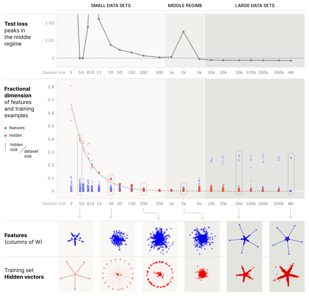
For this suggested replication, we'll look at the Anthropic paper on Double Descent & superposition. This paper ties the phenomena of double descent to models of superposition. The theory posed by this paper goes roughly as follows:

Initially, the model learns a memorising solution where datapoints are represented in superposition. This doesn't generalize, so we get low training loss but high test loss.
Later, the model learns a generalizing solution where features are learned and represented in superposition. This generalizes, so we get low training loss and low test loss.
The spike in loss between these two happens when the model transitions between the memorising and generalizing solutions.

What does it mean to represent datapoints in superposition? If you've done the exercises on correlated / anticorrelated features in an earlier section, you'll know that anticorrelated features are easier to represent in superposition because they don't interfere with each other. This is especially true if features aren't just anticorrelated but are mutually exclusive. From the Anthropic paper:

Consider the case of a language model which verbatim memorizes text. How can it do this? One naive idea is that it might use neurons to create a lookup table mapping sequences to arbitrary continuations. For every sequence of tokens it wishes to memorize, it could dedicate one neuron to detecting that sequence, and then implement arbitrary behavior when it fires. The problem with this approach is that it's extremely inefficient – but it seems like a perfect candidate for superposition, since each case is mutually exclusive and can't interfere.

We'll study this theory in the context of a toy model. Specifically, we'll use the toy model that we worked with in the first section of this paper, but we'll train it in a very particular way: by generating a random batch of data, and then using that same batch for the entire training process. We'll see what happens when the batch sizes change, but the number of features change. According to our theory, the model should represent datapoints in superposition when the batch size is smaller than the number of features, and it should represent features in superposition when the batch size is larger than the number of features.

Rather than giving you a set of exercises to complete, we're leaving this section open-ended. You should consider it more as a paper replication than a set of structured exercises. However, we will give you a few tips:

Rather than using the Adam optimizer, the paper recommends AdamW, with a default weight decay of WEIGHT_DECAY = 1e-2.
- Weight decay constrains the norm of weights, so that they don't grow too large. With no weight decay, we could in theory memorize an arbitrarily large number of datapoints and represent them evenly spaced around the unit circle; then we can perfectly reconstruct them as long as we have a large enough weight vector to project them onto.
The paper recommends a learning rate consisting of a linear warmup up to NUM_WARMUP_STEPS = 2500 (i.e. we increase the learning rate linearly from zero up to LEARNING_RATE = 1e-3), followed by cosine decay until the end of training at NUM_BATCH_UPDATES = 50_000.
The paper recommends using a sparsity of 0.999 for the features, and 10,000 features total. However, we recommend instead using SPARSITY = 0.99 and N_FEATURES = 1000 (following the replication by Marius Hobbhahn). This will cause our model to train faster, while still observing fundamentally the same patterns.
When generating the batch of data, you should normalize it (so each vector for a given batch index & instance has unit norm). The rest of the data generation process should be the same as in the first section of this notebook.
Technically you only need one instance. However, we recommend using a few (e.g. 5-10) so you can pick the instance with lowest loss at the end of training. This is because (thanks to our best frend randomness) not all instances will necessarily learn the optimal solution. In our implementation (code below), we rewrite the optimize function to return (batch_inst, W_inst) at the end, where batch_inst is the batch which had the lowest loss by the end of training, and W_inst are the learned weights for that same instance. This is precisely the data you'll need to make the 2D feature plots featured in the paper.
You can repurpose the function to calculate dimensionality from the section on feature geometry. See the paper for a discussion of a generalized dimensionality function, which doesn't just measure dimensionality of features, but also of datapoints.

To get you started, here are some constants which you might find useful:

NUM_WARMUP_STEPS = 2500
NUM_BATCH_UPDATES = 50_000

WEIGHT_DECAY = 1e-2
LEARNING_RATE = 1e-3

BATCH_SIZES = [3, 5, 6, 8, 10, 15, 30, 50, 100, 200, 500, 1000, 2000]

N_FEATURES = 1000
N_INSTANCES = 5
N_HIDDEN = 2
SPARSITY = 0.99
FEATURE_PROBABILITY = 1 - SPARSITY

Also, if you want some help with the visualisation, the code below will produce the 2D feature visualisations like those found at the bottom of this figure, for all batch sizes stacked horizontally, assuming:

features_list is a list of detached W-matrices for single instances, i.e. each has shape (2, n_features) (these will be used to produce the blue plots on the first row)
data_list is a list of the projections of our batch of data onto the hidden directions of that same instance, i.e. each has shape (2, batch_size) (these will be used to produce the red plots on the second row)

A demonstration is given below (the values are meaningless, they've just been randomly generated to illustrate how to use this function).

features_list = [t.randn(size=(2, 100)) for _ in BATCH_SIZES]
hidden_representations_list = [t.randn(size=(2, batch_size)) for batch_size in BATCH_SIZES]

utils.plot_features_in_2d(
    features_list + hidden_representations_list,
    colors=[["blue"] for _ in range(len(BATCH_SIZES))] + [["red"] for _ in range(len(BATCH_SIZES))],
    title="Double Descent & Superposition (num features = 100)",
    subplot_titles=[f"Features (batch={bs})" for bs in BATCH_SIZES]
    + [f"Data (batch={bs})" for bs in BATCH_SIZES],
    allow_different_limits_across_subplots=True,
    n_rows=2,
)

We've provided an implementation below, although we recommend that you give it a go yourself first before looking at too much of the code. You can use the different dropdowns to get different degrees of hints, if you're struggling.

# YOUR CODE HERE - replicate the results from the Superposition & Deep Double Descent paper!

The first 4 hints give you specific bits of code, if there's any particular part of the implementation you're struggling with:

Hint (basic setup code)

Basic imports and constants:

import math
from typing import Any
import pandas as pd
import plotly.express as px
NUM_WARMUP_STEPS = 2500
NUM_BATCH_UPDATES = 50_000
# EVAL_N_DATAPOINTS = 1_000
WEIGHT_DECAY = 1e-2
LEARNING_RATE = 1e-3
BATCH_SIZES = [3, 4, 5, 6, 8, 10, 15, 20, 30, 50, 100, 200, 300, 500, 1000, 2000, 3000]
# SMALLER_BATCH_SIZES = [3, 6, 10, 30, 100, 500, 2000]
N_FEATURES = 1000
N_INSTANCES = 10
D_HIDDEN = 2
SPARSITY = 0.99
FEATURE_PROBABILITY = 1 - SPARSITY

Our new schedulers, in line with Anthropic's writeup:

def linear_warmup_lr(step, steps):
    """Increases linearly from 0 to 1."""
    return step / steps
def anthropic_lr(step, steps):
    """As per the description in the paper: 2500 step linear warmup, followed by cosine decay to zero."""
    if step < NUM_WARMUP_STEPS:
        return linear_warmup_lr(step, NUM_WARMUP_STEPS)
    else:
        return cosine_decay_lr(step - NUM_WARMUP_STEPS, steps - NUM_WARMUP_STEPS)

Hint (code for new version of ToyModel class)

class DoubleDescentModel(ToyModel):
    W: Float[Tensor, "inst d_hidden feats"]
    b_final: Float[Tensor, "inst feats"]
    # Our linear map (for a single instance) is x -> ReLU(W.T @ W @ x + b_final)
@classmethod
    def dimensionality(
        cls, data: Float[Tensor, "... batch d_hidden"]
    ) -> Float[Tensor, "... batch"]:
        """
        Calculates dimensionalities of data. Assumes data is of shape ... batch d_hidden, i.e. if it's 2D then
        it's a batch of vectors of length d_hidden and we return the dimensionality as a 1D tensor of length
        batch. If it has more dimensions at the start, we assume this means separate calculations for each
        of these dimensions (i.e. they are independent batches of vectors).
        """
        # Compute the norms of each vector (this will be the numerator)
        squared_norms = einops.reduce(data.pow(2), "... batch d_hidden -> ... batch", "sum")
        # Compute the denominator (i.e. get the dot product then sum over j)
        data_normed = data / data.norm(dim=-1, keepdim=True)
        interference = einops.einsum(
            data_normed, data, "... batch_i d_hidden, ... batch_j d_hidden -> ... batch_i batch_j"
        )
        polysemanticity = einops.reduce(
            interference.pow(2), "... batch_i batch_j -> ... batch_i", "sum"
        )
        assert squared_norms.shape == polysemanticity.shape
return squared_norms / polysemanticity
def generate_batch(self, batch_size: int) -> Float[Tensor, "batch inst feats"]:
        """
        New function for generating batch, so we can normalize it.
        """
        # Get batch from prev method
        batch = super().generate_batch(batch_size)
# Normalize the batch (i.e. so each vector for a particular batch & instance has norm 1)
        # (need to be careful about vectors with norm zero)
        norms = batch.norm(dim=-1, keepdim=True)
        norms = t.where(norms.abs() < 1e-6, t.ones_like(norms), norms)
        batch_normed = batch / norms
        return batch_normed
def calculate_loss(
        self,
        out: Float[Tensor, "batch inst feats"],
        batch: Float[Tensor, "batch inst feats"],
        per_inst: bool = False,
    ) -> Float[Tensor, "inst"]:
        """
        New function to calculate loss, because we need a "loss per instance" option to find the best
        instance at the end of our optimization.
        """
        error = self.importance * ((batch - out) ** 2)
        loss = einops.reduce(error, "batch inst feats -> inst", "mean")
        return loss if per_inst else loss.sum()
def optimize(
        self,
        batch_size: int,
        steps: int = NUM_BATCH_UPDATES,
        log_freq: int = 100,
        lr: float = LEARNING_RATE,
        lr_scale: Callable[[int, int], float] = anthropic_lr,
        weight_decay: float = WEIGHT_DECAY,
    ) -> tuple[Tensor, Tensor]:
        optimizer = t.optim.AdamW(list(self.parameters()), lr=lr, weight_decay=weight_decay)
progress_bar = tqdm(range(steps))
# Same batch for each step
        batch = self.generate_batch(batch_size)  # [batch_size inst n_features]
for step in progress_bar:
            # Update learning rate
            step_lr = lr * lr_scale(step, steps)
            for group in optimizer.param_groups:
                group["lr"] = step_lr
# Optimize
            optimizer.zero_grad()
            out = self.forward(batch)
            loss = self.calculate_loss(out, batch)
            loss.backward()
            optimizer.step()
# Display progress bar
            if (step % log_freq == 0) or (step + 1 == steps):
                progress_bar.set_postfix(loss=loss.item() / self.cfg.n_inst, lr=step_lr)
# Generate one final batch to compute the loss (we want only the best instance!)
        with t.inference_mode():
            out = self.forward(batch)
            loss_per_inst = self.calculate_loss(out, batch, per_inst=True)
            best_inst = loss_per_inst.argmin()
            print(f"Best instance = #{best_inst}, with loss {loss_per_inst[best_inst].item():.4e}")
return batch[:, best_inst], self.W[best_inst].detach()

Hint (code to train models & replicate 2D feature plots)

features_list = []
hidden_representations_list = []
for batch_size in tqdm(BATCH_SIZES):
    # Define our model
    cfg = ToyModelConfig(n_features=N_FEATURES, n_inst=N_INSTANCES, d_hidden=D_HIDDEN)
    model = DoubleDescentModel(cfg, feature_probability=FEATURE_PROBABILITY).to(device)
# Optimize, and return the best batch & weight matrix
    batch_inst, W_inst = model.optimize(steps=15_000, batch_size=batch_size)
# Calculate the hidden feature representations, and add both this and weight matrix to our lists of data
    with t.inference_mode():
        hidden = einops.einsum(
            batch_inst, W_inst, "batch features, hidden features -> hidden batch"
        )
    features_list.append(W_inst.cpu())
    hidden_representations_list.append(hidden.cpu())

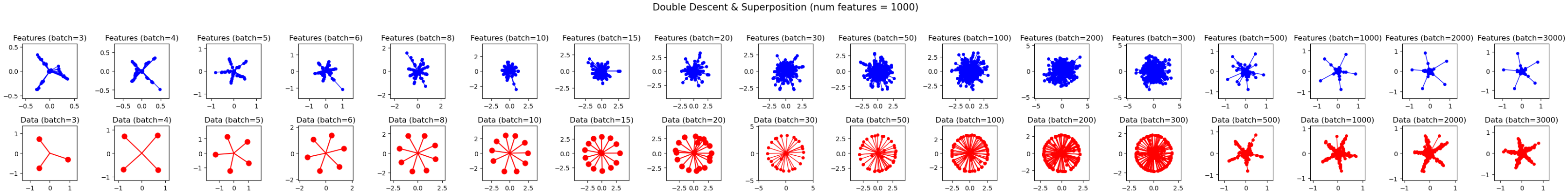
Visualising the 2D feature plots:

utils.plot_features_in_2d(
    features_list + hidden_representations_list,
    colors=[["blue"] for _ in range(len(BATCH_SIZES))] + [["red"] for _ in range(len(BATCH_SIZES))],
    title="Double Descent & Superposition (num features = 1000)",
    subplot_titles=[f"Features (batch={bs})" for bs in BATCH_SIZES] + [f"Data (batch={bs})" for bs in BATCH_SIZES],
    allow_different_limits_across_subplots=True,
    n_rows=2,
)

You should get something like this:

Hint (code to replicate the dimensionality plot)

df_data = {"Batch size": [], "Dimensionality": [], "Data": []}
for batch_size, model_W, hidden in zip(BATCH_SIZES, features_list, hidden_representations_list):
    # Get x-axis data (batch size), and color (blue or red)
    df_data["Batch size"].extend([batch_size]  (N_FEATURES + batch_size))
    df_data["Data"].extend(["features"]  N_FEATURES + ["hidden"]  batch_size)
# Calculate dimensionality of model.W[inst].T, which has shape [d_hidden=2 N_FEATURES]
    feature_dim = DoubleDescentModel.dimensionality(model_W.T)
    assert feature_dim.shape == (N_FEATURES,)
# Calculate dimensionality of model's batch data hidden representation. This has shape [d_hidden=2 batch_size]
    data_dim = DoubleDescentModel.dimensionality(hidden.T)
    assert data_dim.shape == (batch_size,)
# Add them both to the data
    df_data["Dimensionality"].extend(feature_dim.tolist() + data_dim.tolist())
df = pd.DataFrame(df_data)
eps = 0.01
xline1, xline2 = (100  200) ** 0.5, (500 * 1000) ** 0.5
vrect_kwargs: dict[str, Any] = dict(opacity=0.5, layer="below", line_width=0)
xrange = [math.log10(1.5), math.log10(5000)]
fig = (
    px.strip(
        df,
        x="Batch size",
        y="Dimensionality",
        color="Data",
        color_discrete_sequence=["rgba(0,0,255,0.3)", "rgba(255,0,0,0.3)"],
        log_x=True,
        template="simple_white",
        width=1000,
        height=600,
        title="Dimensionality of features & hidden representation of training examples",
    )
    .update_traces(marker=dict(opacity=0.5))
    .update_layout(
        xaxis=dict(range=xrange, tickmode="array", tickvals=BATCH_SIZES),
        yaxis=dict(range=[-0.05, 1.0]),
    )
    .add_vrect(x0=1, x1=(1 - eps) * xline1, fillcolor="#ddd", **vrect_kwargs)
    .add_vrect(x0=(1 + eps)  xline1, x1=(1 - eps)  xline2, fillcolor="#ccc", **vrect_kwargs)
    .add_vrect(x0=(1 + eps) * xline2, x1=10_000, fillcolor="#bbb", **vrect_kwargs)
    .add_scatter(
        x=BATCH_SIZES,
        y=[2 / b for b in BATCH_SIZES],
        mode="lines",
        line=dict(shape="spline", dash="dot", color="#333", width=1),
        name="d_hidden / batch_size",
    )
)
fig.show()

You should get something like this:

Lastly, you get the full solution code here:

Solution (full)

import math
from typing import Any
import pandas as pd
import plotly.express as px
NUM_WARMUP_STEPS = 2500
NUM_BATCH_UPDATES = 50_000
# EVAL_N_DATAPOINTS = 1_000
WEIGHT_DECAY = 1e-2
LEARNING_RATE = 1e-3
BATCH_SIZES = [3, 4, 5, 6, 8, 10, 15, 20, 30, 50, 100, 200, 300, 500, 1000, 2000, 3000]
# SMALLER_BATCH_SIZES = [3, 6, 10, 30, 100, 500, 2000]
N_FEATURES = 1000
N_INSTANCES = 10
D_HIDDEN = 2
SPARSITY = 0.99
FEATURE_PROBABILITY = 1 - SPARSITY
def linear_warmup_lr(step, steps):
    """Increases linearly from 0 to 1."""
    return step / steps
def anthropic_lr(step, steps):
    """As per the description in the paper: 2500 step linear warmup, followed by cosine decay to zero."""
    if step < NUM_WARMUP_STEPS:
        return linear_warmup_lr(step, NUM_WARMUP_STEPS)
    else:
        return cosine_decay_lr(step - NUM_WARMUP_STEPS, steps - NUM_WARMUP_STEPS)
class DoubleDescentModel(ToyModel):
    W: Float[Tensor, "inst d_hidden feats"]
    b_final: Float[Tensor, "inst feats"]
    # Our linear map (for a single instance) is x -> ReLU(W.T @ W @ x + b_final)
@classmethod
    def dimensionality(
        cls, data: Float[Tensor, "... batch d_hidden"]
    ) -> Float[Tensor, "... batch"]:
        """
        Calculates dimensionalities of data. Assumes data is of shape ... batch d_hidden, i.e. if
        it's 2D then it's a batch of vectors of length d_hidden and we return the dimensionality
        as a 1D tensor of length batch. If it has more dimensions at the start, we assume this
        means separate calculations for each of these dimensions (i.e. they are independent batches
        of vectors).
        """
        # Compute the norms of each vector (this will be the numerator)
        squared_norms = einops.reduce(data.pow(2), "... batch d_hidden -> ... batch", "sum")
        # Compute the denominator (i.e. get the dot product then sum over j)
        data_normed = data / data.norm(dim=-1, keepdim=True)
        interference = einops.einsum(
            data_normed, data, "... batch_i d_hidden, ... batch_j d_hidden -> ... batch_i batch_j"
        )
        polysemanticity = einops.reduce(
            interference.pow(2), "... batch_i batch_j -> ... batch_i", "sum"
        )
        assert squared_norms.shape == polysemanticity.shape
return squared_norms / polysemanticity
def generate_batch(self, batch_size: int) -> Float[Tensor, "batch inst feats"]:
        """
        New function for generating batch, so we can normalize it.
        """
        # Get batch from prev method
        batch = super().generate_batch(batch_size)
# Normalize the batch (i.e. so each vector for a particular batch & instance has norm 1)
        # (need to be careful about vectors with norm zero)
        norms = batch.norm(dim=-1, keepdim=True)
        norms = t.where(norms.abs() < 1e-6, t.ones_like(norms), norms)
        batch_normed = batch / norms
        return batch_normed
def calculate_loss(
        self,
        out: Float[Tensor, "batch inst feats"],
        batch: Float[Tensor, "batch inst feats"],
        per_inst: bool = False,
    ) -> Float[Tensor, "inst"]:
        """
        New function to calculate loss, because we need a "loss per instance" option to find the
        best instance at the end of our optimization.
        """
        error = self.importance * ((batch - out) ** 2)
        loss = einops.reduce(error, "batch inst feats -> inst", "mean")
        return loss if per_inst else loss.sum()
def optimize(
        self,
        batch_size: int,
        steps: int = NUM_BATCH_UPDATES,
        log_freq: int = 100,
        lr: float = LEARNING_RATE,
        lr_scale: Callable[[int, int], float] = anthropic_lr,
        weight_decay: float = WEIGHT_DECAY,
    ) -> tuple[Tensor, Tensor]:
        optimizer = t.optim.AdamW(list(self.parameters()), lr=lr, weight_decay=weight_decay)
progress_bar = tqdm(range(steps))
# Same batch for each step
        batch = self.generate_batch(batch_size)  # [batch_size inst n_features]
for step in progress_bar:
            # Update learning rate
            step_lr = lr  lr_scale(step, steps)
            for group in optimizer.param_groups:
                group["lr"] = step_lr
# Optimize
            optimizer.zero_grad()
            out = self.forward(batch)
            loss = self.calculate_loss(out, batch)
            loss.backward()
            optimizer.step()
# Display progress bar
            if (step % log_freq == 0) or (step + 1 == steps):
                progress_bar.set_postfix(loss=loss.item() / self.cfg.n_inst, lr=step_lr)
# Generate one final batch to compute the loss (we want only the best instance!)
        with t.inference_mode():
            out = self.forward(batch)
            loss_per_inst = self.calculate_loss(out, batch, per_inst=True)
            best_inst = loss_per_inst.argmin()
            print(f"Best instance = #{best_inst}, with loss {loss_per_inst[best_inst].item():.4e}")
return batch[:, best_inst], self.W[best_inst].detach()
# ! Results, part 1/2
features_list = []
hidden_representations_list = []
for batch_size in tqdm(BATCH_SIZES):
    # Define our model
    cfg = ToyModelConfig(n_features=N_FEATURES, n_inst=N_INSTANCES, d_hidden=D_HIDDEN)
    model = DoubleDescentModel(cfg, feature_probability=FEATURE_PROBABILITY).to(device)
# Optimize, and return the best batch & weight matrix
    batch_inst, W_inst = model.optimize(steps=15_000, batch_size=batch_size)
# Calculate the hidden feature representations, and add both this and weight matrix to our
    # lists of data
    with t.inference_mode():
        hidden = einops.einsum(
            batch_inst, W_inst, "batch features, hidden features -> hidden batch"
        )
    features_list.append(W_inst.cpu())
    hidden_representations_list.append(hidden.cpu())
utils.plot_features_in_2d(
    features_list + hidden_representations_list,
    colors=[["blue"] for _ in range(len(BATCH_SIZES))]
    + [["red"] for _ in range(len(BATCH_SIZES))],
    title="Double Descent & Superposition (num features = 1000)",
    subplot_titles=[f"Features (batch={bs})" for bs in BATCH_SIZES]
    + [f"Data (batch={bs})" for bs in BATCH_SIZES],
    allow_different_limits_across_subplots=True,
    n_rows=2,
)
# ! Results, part 2/2
df_data = {"Batch size": [], "Dimensionality": [], "Data": []}
for batch_size, model_W, hidden in zip(BATCH_SIZES, features_list, hidden_representations_list):
    # Get x-axis data (batch size), and color (blue or red)
    df_data["Batch size"].extend([batch_size]  (N_FEATURES + batch_size))
    df_data["Data"].extend(["features"]  N_FEATURES + ["hidden"]  batch_size)
# Calculate dimensionality of model.W[inst].T, which has shape [d_hidden=2 N_FEATURES]
    feature_dim = DoubleDescentModel.dimensionality(model_W.T)
    assert feature_dim.shape == (N_FEATURES,)
# Calculate dimensionality of model's batch data hidden representation.
    # This has shape [d_hidden=2 batch_size]
    data_dim = DoubleDescentModel.dimensionality(hidden.T)
    assert data_dim.shape == (batch_size,)
# Add them both to the data
    df_data["Dimensionality"].extend(feature_dim.tolist() + data_dim.tolist())
df = pd.DataFrame(df_data)
eps = 0.01
xline1, xline2 = (100 * 200) ** 0.5, (500 * 1000) ** 0.5
vrect_kwargs: dict[str, Any] = dict(opacity=0.5, layer="below", line_width=0)
xrange = [math.log10(1.5), math.log10(5000)]
fig = (
    px.strip(
        df,
        x="Batch size",
        y="Dimensionality",
        color="Data",
        color_discrete_sequence=["rgba(0,0,255,0.3)", "rgba(255,0,0,0.3)"],
        log_x=True,
        template="simple_white",
        width=1000,
        height=600,
        title="Dimensionality of features & hidden representation of training examples",
    )
    .update_traces(marker=dict(opacity=0.5))
    .update_layout(
        xaxis=dict(range=xrange, tickmode="array", tickvals=BATCH_SIZES),
        yaxis=dict(range=[-0.05, 1.0]),
    )
    .add_vrect(x0=1, x1=(1 - eps) * xline1, fillcolor="#ddd", **vrect_kwargs)
    .add_vrect(x0=(1 + eps)  xline1, x1=(1 - eps)  xline2, fillcolor="#ccc", **vrect_kwargs)
    .add_vrect(x0=(1 + eps) * xline2, x1=10_000, fillcolor="#bbb", **vrect_kwargs)
    .add_scatter(
        x=BATCH_SIZES,
        y=[2 / b for b in BATCH_SIZES],
        mode="lines",
        line=dict(shape="spline", dash="dot", color="#333", width=1),
        name="d_hidden / batch_size",
    )
)
fig.show()