3️⃣ Feature Geometry

Learning Objectives

• Learn about dimensionality, which essentially measures what fraction of a dimension is allocated to a specific feature
• Understand the geometric intuitions behind superposition, and how they relate to the more general ideas of superposition in larger models

Note - this section is optional, since it goes into quite extreme detail about the specific problem setup we're using here. If you want, you can jump to the next section.

Dimensionality

We've seen that superposition can allow a model to represent extra features, and that the number of extra features increases as we increase sparsity. In this section, we'll investigate this relationship in more detail, discovering an unexpected geometric story: features seem to organize themselves into geometric structures such as pentagons and tetrahedrons!

The code below runs a third experiment, with all importances the same. We're first interested in the number of features the model has learned to represent. This is well represented with the squared Frobenius norm of the weight matrix $W$, i.e. $||W||_F^2 = \sum_{ij}W_{ij}^2$.

If you run the code below, you'll also plot the total number of "dimensions per feature", $m/\big\|W\big\|_F^2$.

cfg = ToyModelConfig(n_features=200, d_hidden=20, n_inst=20)

# For this experiment, use constant importance across features (but still vary sparsity across instances)
feature_probability = 20 ** -t.linspace(0, 1, cfg.n_inst)

model = ToyModel(
    cfg=cfg,
    device=device,
    feature_probability=feature_probability[:, None],
)
model.optimize(steps=10_000)


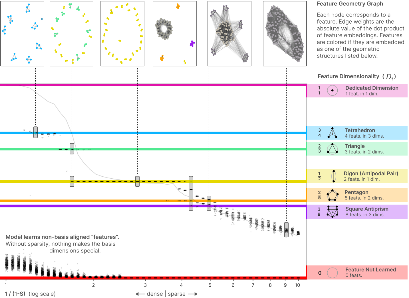
utils.plot_feature_geometry(model)

Surprisingly, we find that this graph is "sticky" at $1$ and $1/2$. On inspection, the $1/2$ "sticky point" seems to correspond to a precise geometric arrangement where features come in "antipodal pairs", each being exactly the negative of the other, allowing two features to be packed into each hidden dimension. It appears that antipodal pairs are so effective that the model preferentially uses them over a wide range of the sparsity regime.

It turns out that antipodal pairs are just the tip of the iceberg. Hiding underneath this curve are a number of extremely specific geometric configurations of features.

How can we discover these geometric configurations? Consider the following metric, which the authors named the dimensionality of a feature:

Intuitively, this is a measure of what "fraction of a dimension" a specific feature gets. Let's try and get a few intuitions for this metric:

• It's never less than zero.
  • It's equal to zero if and only if the vector is the zero vector, i.e. the feature isn't represented.
• It's never greater than one (because when $j = i$, the term in the denominator sum is equal to the numerator).
  • It's equal to one if and only if the $i$-th feature vector $W_i$ is orthogonal to all other features (because then $j=i$ is the only term in the denominator sum).
  • Intuitively, in this case the feature has an entire dimension to itself.
• If there are $k$ features which are all parallel to each other, and orthogonal to all others, then they "share" the dimensionality equally, i.e. $D_i = 1/k$ for each of them.
• The sum of all $D_i$ can't be greater than the total number of features $m$, with equality if and only if all the vectors are orthogonal.

Exercise - compute dimensionality

Remember, $W$ has shape (n_inst, d_hidden, n_features). The vectors $W_i$ refer to the feature vectors (i.e. they have length d_hidden), and you should broadcast your calculations over the n_inst dimension.

@t.inference_mode()
def compute_dimensionality(
    W: Float[Tensor, "n_inst d_hidden n_features"],
) -> Float[Tensor, "n_inst n_features"]:
    raise NotImplementedError()


tests.test_compute_dimensionality(compute_dimensionality)

@t.inference_mode()
def compute_dimensionality(
    W: Float[Tensor, "n_inst d_hidden n_features"],
) -> Float[Tensor, "n_inst n_features"]:
    W_norms = W.norm(dim=1, keepdim=True)
    numerator = W_norms.squeeze() ** 2
# Compute denominator terms
    W_normalized = W / (W_norms + 1e-8)
    denominator = einops.einsum(W_normalized, W, "i h f1, i h f2 -> i f1 f2").pow(2).sum(-1)
return numerator / denominator

The code below plots the fractions of dimensions, as a function of increasing levels of sparsity across our instances.

W = model.W.detach()
dim_fracs = compute_dimensionality(W)

utils.plot_feature_geometry(model, dim_fracs=dim_fracs)

What's going on here? It turns out that the model likes to create specific weight geometries and kind of jumps between the different configurations. For example:

• With zero (or very small) sparsity, the feature basis isn't privileged by anything, and so the model represents features with arbitrary directions instead. There's no reason for some features to be represented faithfully and others not to be.
• When we get to higher levels of sparsity, the feature basis becomes privileged. So the model phase-transitions to representing some features in antipodal pairs, and the rest aren't interpreted.
• With further increases in sparsity, we transition to different geometries (see diagram below).

The moral? Superposition is very hard to pin down! There are many points between a dimensionality of 0 (not learning a feature) and 1 (dedicating a dimension to a feature). As an analogy, we often think of water as only having three phases: ice, water and steam. But this is a simplification: there are actually many phases of ice, often corresponding to different crystal structures (eg. hexagonal vs cubic ice). In a vaguely similar way, neural network features seem to also have many other phases within the general category of "superposition."

Note that we should take care not to read too much significance into these results. A lot of it depends delicately on the details of our experimental setup (e.g. we used $W^T W$, a positive semidefinite matrix, and there's a correspondence between low-dimensional symmetric pos-semidef matrices like these and the kinds of polytopes that we've seen in the plots above). But hopefully this has given you a sense of the relevant considerations when it comes to packing features into fewer dimensions.