3️⃣ Neuron Interpretability: A Deep Dive

Learning Objectives

• Apply direct logit attribution to understand how a neuron's output weights directly effect predictions
• Use SVD-based techniques to assess how much of a neuron's input/output behaviour is captured by some subspace
• Use techniques like max activating datasets and spectrum plots, and understand their strengths and limitations

To practice neuron interpretability, let's take a deep dive into understanding this neuron - the techniques and code should transfer pretty well to any other neurons!

The spirit of this section is to practice doing various standard things that you could go and apply to another neuron in practice - I end it still being fairly confused, and with many dangling threads!

As above, we can use the probe weights to analyse its input weights. So we go in with the hypothesis that it detects (C0==BLANK) & (D1==THEIRS) & (E2==MINE), and that it directly boosts the C0 logit - this configuration means that C0 must be legal, because it would flank D1 along the diagonal!

Direct logit attribution

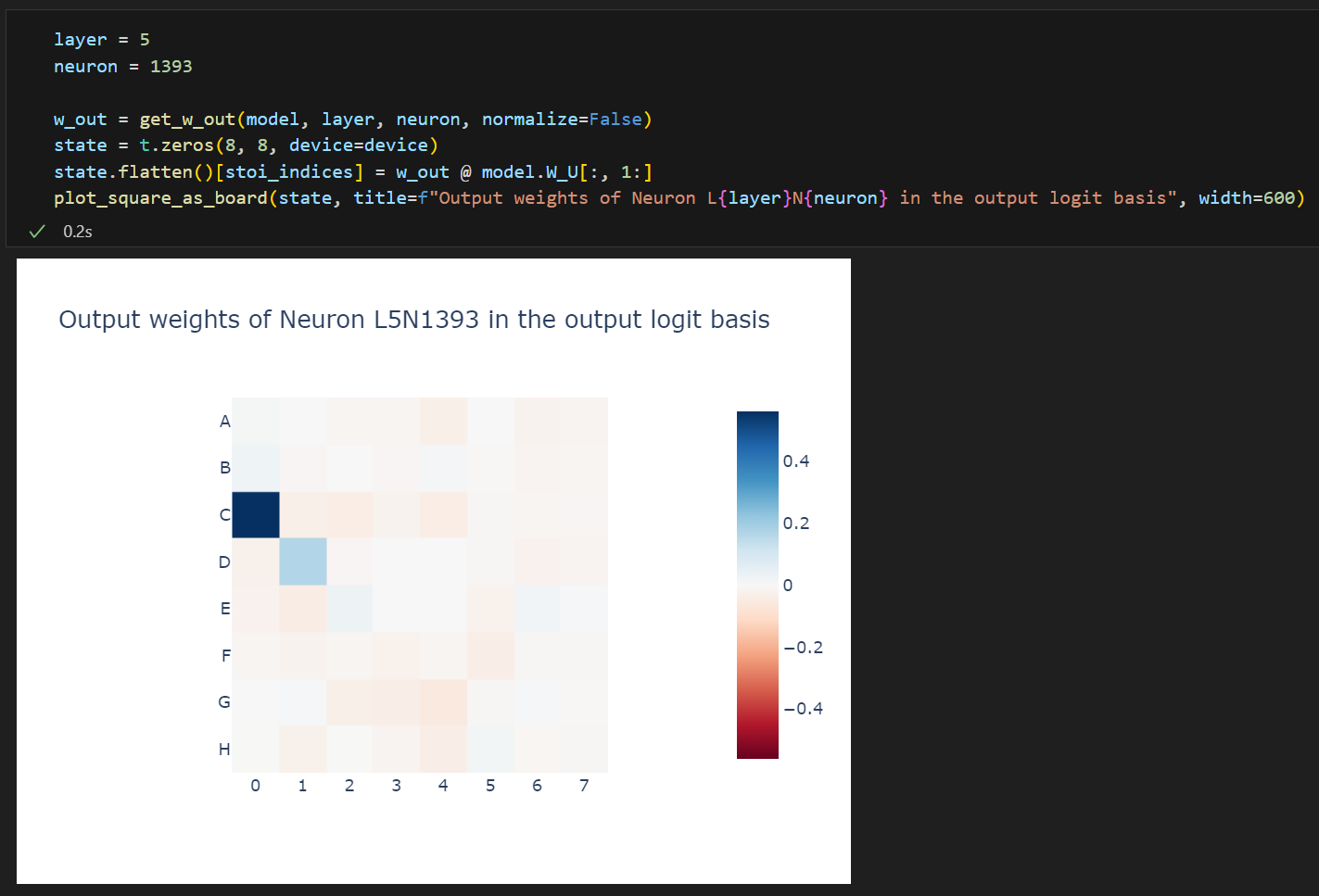
As we studied briefly in the previous section, we can look at the direct logit attribution of a neuron's output weights - i.e. w_out @ W_U, to see if the neuron significantly affects the output logits directly. Note that this is purely weights based analysis, we're not yet looking at actual model activations.

layer = 5
neuron = 1393

# Get neuron output weights in unembedding basis
w_out = get_w_out(model, layer, neuron, normalize=False)
w_out_W_U_basis = w_out @ model.W_U[:, 1:]  # shape (60,)

# Turn into a (rows, cols) tensor, using indexing
w_out_W_U_basis_rearranged = t.zeros((8, 8), device=device)
w_out_W_U_basis_rearranged.flatten()[ALL_SQUARES] = w_out_W_U_basis

# Plot results
utils.plot_board_values(
    w_out_W_U_basis_rearranged,
    title=f"Cosine sim of neuron L{layer}N{neuron} with W<sub>U</sub> directions",
    width=450,
    height=380,
)

Here we immediately see that boosting C0 is an important part of what happens (which fits with our earlier hypothesis about the diagonal pattern which this MLP was picking up on), but that it also boosts D1, which is surprising! (D1 is filled in our hypothesis, so must be illegal!)

One hypothesis is that the unembed for C0 and D1 are highly aligned, so it can't easily boost one but not the other.

Exercise - compare the unembeds for C0 and D1

Is this hypothesis true? Test it by calculating the cosine similarity of the C0 and D1 unembeds.

Recall, you can use the utils.label_to_id helper function to convert a label like "C0" to an integer index (which you can use to index into the unembedding).

# YOUR CODE HERE - calculate cosine sim between unembeddings

c0_U = model.W_U[:, utils.label_to_id("C0")].detach()
c0_U /= c0_U.norm()
d1_U = model.W_U[:, utils.label_to_id("D1")].detach()
d1_U /= d1_U.norm()
print(f"Cosine sim of C0 and D1 unembeds: {c0_U @ d1_U:.3f}")

To check that this is a big part of the neuron's output, lets look at the fraction of variance of the output captured by the $W_U$ subspace.

Exercise - compute fraction of variance explained by unembedding subspace

Note - when we say "fraction of a vector's variance explained by a subspace", this means the fraction of the original vector's squared norm which is represented by its projection onto the subspace. So if we have a vector $v$ and a subspace $W$ represented by a matrix of orthogonal row vectors, then $v^T W$ are the components of the projection of $v$ onto $W$, and the fraction of $v$'s variance explained by the subspace $W$ is $\|v^T W\|^2 / \|v\|^2$.

If you're confused by this, then you should go to the How much variance does the probe explain? section, where we do a computation which is similar to (but more complicated than) to the one which you should do now.

Gotcha - remember to remove the 0th vocab entry from $W_U$ before taking SVD, since this corresponds to the "pass" move which never comes up in our data.

# YOUR CODE HERE - compute the variance frac of neuron output vector explained by unembedding subspace

w_out = get_w_out(model, layer, neuron, normalize=True)
U, S, Vh = t.svd(model.W_U[:, 1:])
print(f"Fraction of variance captured by W_U: {((w_out @ U).norm().item() ** 2):.4f}")

Fraction of variance captured by W_U: 0.2868

Another quick sanity check is just plotting what the neuron activations look like over the 50 games in our cache - we see that it only matters in a few games, and matters every other move (which makes sense for a feature denominated in terms of my vs their colours - this alternates every move as the colours swap!)

neuron_acts = focus_cache["post", layer, "mlp"][:, :, neuron]

fig = px.imshow(
    to_numpy(neuron_acts),
    title=f"L{layer}N{neuron} Activations over 50 games",
    labels={"x": "Move", "y": "Game"},
    color_continuous_scale="RdBu",
    color_continuous_midpoint=0.0,
    aspect="auto",
    width=900,
    height=400,
)
fig.show()

Exercise - figure out what's going on with one of these games

Take one of the games where this neuron fires (e.g. game 5 seems like a good example). Plot the state of the game using plot_board_values (you can take code from earlier in this notebook).

imshow(
    focus_states[5, :25],
    facet_col=0,
    facet_col_wrap=5,
    y=list("ABCDEFGH"),
    facet_labels=[f"Move {i}" for i in range(25)],
    title="First 16 moves of first game",
    color_continuous_scale="Greys",
    coloraxis_showscale=False,
    width=1000,
    height=1000,
)

Max Activating Datasets

Max activating datasets are a useful but also sometimes misleading tool we can use to better understand a neuron's activations. From my Dynalist notes:

• Max Activating Dataset Examples aka dataset examples aka max examples are a simple technique for neuron interpretability. The model is run over a lot of data points, and we select the top K data points by how much they activate that neuron.
  • Sometimes there is a clear pattern in these inputs (eg they’re all pictures of boats), and this is (weak!) evidence that the neuron detects that pattern. Sometimes there are multiple clusters of inputs according to different patterns, which suggests that the neuron is polysemantic (i.e. it represents some combination of multiple different features).
  • This is a very simple and dumb technique, and has faced criticism, see e.g. The Interpretability Illusion which found that different datasets gave different sets of examples, each of which had a different clear pattern.
  • See outputs of this for image models in OpenAI Microscope and language models in Neuroscope.

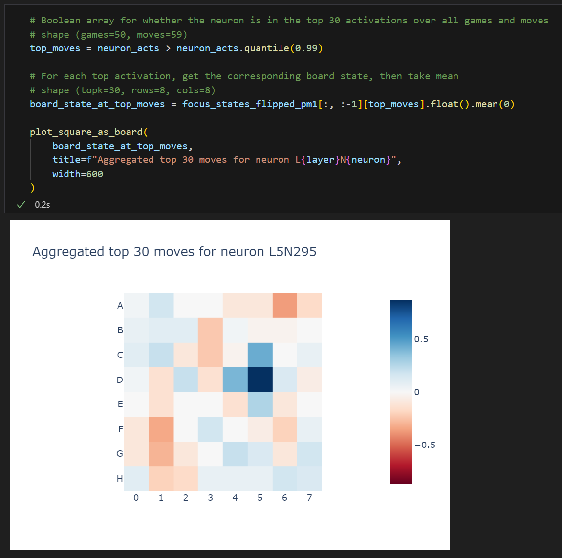
Doing this properly across many games is effort, but here we have cached outputs on 50 games (3000 moves), so we can look at the top 30 games there.

# Get top 30 games & plot them all
top_moves = neuron_acts > neuron_acts.quantile(0.99)
top_focus_states = focus_states[:, :-1][top_moves.cpu()]
top_focus_states_flip = focus_states_theirs_vs_mine[:, :-1][top_moves.cpu()]
utils.plot_board_values(
    top_focus_states,
    boards_per_row=10,
    board_titles=[f"{act=:.2f}" for act in neuron_acts[top_moves]],
    title=f"Top 30 moves for neuron L{layer}N{neuron}",
    width=1600,
    height=500,
)

# Plot heatmaps for how frequently any given square is mine/theirs/blank in those top 30
utils.plot_board_values(
    t.stack([top_focus_states_flip == 0, top_focus_states_flip == 1, top_focus_states_flip == 2]).float().mean(1),
    board_titles=["Blank", "Theirs", "Mine"],
    title=f"Aggregated top 30 moves for neuron L{layer}N{neuron}, in 'blank/mine/theirs' basis",
    width=800,
    height=380,
)

Note that the blank cells show up with high frequency - this is one of the kinds of things you have to watch out for, since exactly how you've defined your dataset will affect the features of the max activating dataset you end up finding (and it might be the case that each dataset exhibits a clear but misleading pattern).

We mostly care about the "mine vs theirs" distinction here because it's the most interesting, so let's create a new tensor where "mine" is -1 and "theirs" is +1, then taking a mean over this tensor will give us an idea of "mine vs theirs".

focus_states_theirs_vs_mine_pm1 = t.zeros_like(focus_states_theirs_vs_mine, device=device)
focus_states_theirs_vs_mine_pm1[focus_states_theirs_vs_mine == 2] = 1
focus_states_theirs_vs_mine_pm1[focus_states_theirs_vs_mine == 1] = -1

board_state_at_top_moves = focus_states_theirs_vs_mine_pm1[:, :-1][top_moves].float().mean(0)
board_state_at_top_moves.shape

utils.plot_board_values(
    board_state_at_top_moves,
    title=f"Aggregated top 30 moves for neuron L{layer}N{neuron}<br>(1 = theirs, -1 = mine)",
    height=380,
    width=450,
)

Exercise - investigate more neurons

We see that, for all moves in the max activating dataset, D1 is theirs and E2 is mine. This is moderately strong evidence that our neuron is doing the thing we think it's doing.

Let's review the kinds of plots we've made during this section. There have been two kinds:

1. Direct logit attribution plots, where we calculated the cosine similarity of the corresponding neuron with the unembedding weights corresponding to each square.

Example

1. Max activating dataset plots, where we get a heatmap of how frequently a square was mine / theirs over the dataset we're choosing (where that dataset is the max activating dataset for some particular neuron).

Example

Try and make both of these plots, but for all the top 10 neurons in layer 5 (where, like before, we measure "top 10" by the standard deviation of the neurons' activations, over all games and moves from the data in focus_cache). You'll be able to copy and paste some code from earlier.

We've given you the code for making the plots. All you need to do is calculate the output_weights_in_logit_basis and board_states tensors, which should be batched versions of the tensors which were used to generate the plots above (the 0th axis should be the neuron index, i.e. the [0, ...]-th slice of each of these tensors should be the things we fed into our plotting functions earlier in this section).

Can you guess what any of these neurons are doing? Does it help if you also plot some of them in the logit basis, like you did for L5N1393?

# YOUR CODE HERE - investigate the top 10 neurons by std dev of activations, see what you can find!

layer = 5
top_neurons = focus_cache["post", layer].std(dim=[0, 1]).argsort(descending=True)[:10]
board_states = []
output_weights_in_logit_basis = []
for neuron in top_neurons:
    # Get output weights in logit basis
    w_out = get_w_out(model, layer, neuron, normalize=False)
    state = t.zeros(8, 8, device=device)
    state.flatten()[ALL_SQUARES] = w_out @ model.W_U[:, 1:]
    output_weights_in_logit_basis.append(state)
# Get max activating dataset aggregations
    neuron_acts = focus_cache["post", 5, "mlp"][:, :, neuron]
    top_moves = neuron_acts > neuron_acts.quantile(0.99)
    board_state_at_top_moves = focus_states_theirs_vs_mine_pm1[:, :-1][top_moves].float().mean(0)
    board_states.append(board_state_at_top_moves)
output_weights_in_logit_basis = t.stack(output_weights_in_logit_basis)
board_states = t.stack(board_states)
utils.plot_board_values(
    output_weights_in_logit_basis,
    title=f"Output weights of top 10 neurons in layer {layer}, in the output logit basis",
    board_titles=[f"L{layer}N{n.item()}" for n in top_neurons],
    width=1600,
    height=360,
)
utils.plot_board_values(
    board_states,
    title=f"Aggregated top 30 moves for each top 10 neuron in layer {layer}",
    board_titles=[f"L{layer}N{n.item()}" for n in top_neurons],
    width=1600,
    height=360,
)

How do you interpret the results?

Spectrum Plots

One of the best ways to validate a hypothesis about neurons is to use a spectrum plot, where we plot a histogram of the neuron activations across the full data distribution (or at least some random sample) and categorise each activation by whether it has the property we think the neuron is detecting. We can do a janky version of that with the neuron's activations on our 50 games (plotting each histogram group as percent of the group size, to normalise for most games not having the configuration hypothesised).

Fascinatingly, we see that our hypothesis did not fully capture the neuron - almost every high activation had the hypothesised configuration, but so did some low ones! I'm not sure what's going on here, but it reveals a weakness of max activating dataset examples - they don't let you notice when your hypothesis allows false positives!

c0 = focus_states_theirs_vs_mine_pm1[:, :, 2, 0]
d1 = focus_states_theirs_vs_mine_pm1[:, :, 3, 1]
e2 = focus_states_theirs_vs_mine_pm1[:, :, 4, 2]

label = (c0 == 0) & (d1 == -1) & (e2 == 1)

neuron_acts = focus_cache["post", 5][:, :, 1393]


def make_spectrum_plot(neuron_acts: Float[Tensor, "batch"], label: Bool[Tensor, "batch"], **kwargs) -> None:
    """
    Generates a spectrum plot from the neuron activations and a set of labels.
    """
    px.histogram(
        pd.DataFrame({"acts": neuron_acts.tolist(), "label": label.tolist()}),
        x="acts",
        color="label",
        histnorm="percent",
        barmode="group",
        color_discrete_sequence=px.colors.qualitative.Bold,
        nbins=100,
        **kwargs,
    ).show()


make_spectrum_plot(
    neuron_acts.flatten(),
    label[:, :-1].flatten(),
    title="Spectrum plot for neuron L5N1393 testing C0==BLANK & D1==THEIRS & E2==MINE",
    width=1200,
    height=400,
)

Exercise - investigate this spectrum plot

Look at the moves with this configuration and low activations - what's going on there? Can you see any patterns in the board states? In the moves? What does the neuron activation look like over the course of the game?

Exercise - make more spectrum plots

Try to find another neuron with an interpretable attention pattern. Make a spectrum plot for it. What do you find?

Recap of this section

In this section, we did the following:

• Used direct logit attribution to see how the output weights of neurons were affecting the output logits for each square.
  • Found L5N1393 was boosting the logits for cell C0.
• Used max activating datasets to see which kinds of game states were causing certain neurons to fire strongly.
  • Found L5N1393 was firing strongly when on the (C0==BLANK) & (D1==THEIRS) & (E2==MINE) pattern.
• Repeated these two plots for a bunch of other neurons, and found that lots of them were interpretable in similar ways (i.e. they all activated strongly on a particular pattern, and positively affected the logits for a square which would be legal to play in that pattern).
• Made a spectrum plot, and found that our explanation of the neuron wasn't the whole story (some game states with the given pattern didn't cause the neuron to fire).
  • This revealed a weakness with max activating datasets as a method of finding a full explanation of a neuron's behaviour.