2️⃣ Looking for modular circuits

Learning Objectives

• Learn how to use our linear probe across multiple layers
• Apply activation patching at a given sequence position to test hypotheses about our model
• Understand how a neuron can be characterized in terms of its input and output weights

Probing Across Layers

The probe's inputs are accumulated in the residual stream over the six layers - the residual stream is the sum of the output of each previous head and neuron. We can therefore analyse which previous model components most contribute to the overall probe computation, and use this to identify the end of the world model computing circuit.

Let's analyse move 20 in game 1, where we can see that the probe has perfect accuracy after layer 6.

layer = 6
game_index = 1
move = 20

utils.plot_board_values(
    focus_states[game_index, move],
    text=focus_legal_moves_annotation[game_index][move],
    title=f"Focus game #{game_index}, board after move {move}",
    width=400,
    height=400,
)

plot_probe_outputs(focus_cache, linear_probe, layer, game_index, move, title=f"Probe outputs (layer {layer})")

We now plot the contributions of the attention and MLP layers to the my_probe direction. Strikingly, we see that the MLP layers are important for the vertical stripe that we just taken by the opponent, but that most of the rest seems to be done by the attention layers.

Exercise - compute attn and mlp contributions

Below, you should define attn_contributions and mlp_contributions. You should do this by taking the batched dot product of the vectors written to the residual stream in each layer (from layer 0 to layer layer inclusive), and the probe direction "my vs their" which you computed earlier (i.e. my_probe).

Note, we're looking for the marginal contribution to the probe direction from each of our components, not the accumulated residual stream. This is because we want to see which components have a strong effect on the output.

def calculate_attn_and_mlp_probe_score_contributions(
    focus_cache: ActivationCache,
    probe: Float[Tensor, "d_model rows cols"],
    layer: int,
    game_index: int,
    move: int,
) -> tuple[Float[Tensor, "layers rows cols"], Float[Tensor, "layers rows cols"]]:
    # YOUR CODE HERE - define `attn_contributions` and `mlp_contributions` using the cache & probe

    return (attn_contributions, mlp_contributions)


layer = 6
attn_contributions, mlp_contributions = calculate_attn_and_mlp_probe_score_contributions(
    focus_cache, my_probe, layer, game_index, move
)

utils.plot_board_values(
    mlp_contributions,
    title=f"MLP Contributions to my vs their (game #{game_index}, move {move})",
    board_titles=[f"Layer {i}" for i in range(layer + 1)],
    width=1400,
    height=340,
)
utils.plot_board_values(
    attn_contributions,
    title=f"Attn Contributions to my vs their (game #{game_index}, move {move})",
    board_titles=[f"Layer {i}" for i in range(layer + 1)],
    width=1400,
    height=340,
)

def calculate_attn_and_mlp_probe_score_contributions(
    focus_cache: ActivationCache,
    probe: Float[Tensor, "d_model rows cols"],
    layer: int,
    game_index: int,
    move: int,
) -> tuple[Float[Tensor, "layers rows cols"], Float[Tensor, "layers rows cols"]]:
    attn_contributions = einops.einsum(
        t.stack([focus_cache["attn_out", l][game_index, move] for l in range(layer + 1)]),
        probe,
        "layers d_model, d_model rows cols -> layers rows cols",
    )
    mlp_contributions = einops.einsum(
        t.stack([focus_cache["mlp_out", l][game_index, move] for l in range(layer + 1)]),
        probe,
        "layers d_model, d_model rows cols -> layers rows cols",
    )
return (attn_contributions, mlp_contributions)

Next, you should return (and plot) overall probe scores (i.e. from the accumulated residual stream by the end of layer layer). The code should be similar to the code you wrote immediately above, except you're taking the value at the residual stream up to and including layer layer, rather than the MLP or attention contributions.

def calculate_accumulated_probe_score(
    focus_cache: ActivationCache,
    probe: Float[Tensor, "d_model rows cols"],
    layer: int,
    game_index: int,
    move: int,
) -> Float[Tensor, "layers rows cols"]:
    # YOUR CODE HERE - define `attn_contributions` and `mlp_contributions` using the cache & probe

    return residual_stream_score


residual_stream_score = calculate_accumulated_probe_score(focus_cache, my_probe, layer, game_index, move)

utils.plot_board_values(
    residual_stream_score,
    title=f"Residual stream probe values for 'my vs their' (game #{game_index}, move {move})",
    board_titles=[f"Layer {i}" for i in range(layer + 1)],
    width=1400,
    height=340,
)

def calculate_accumulated_probe_score(
    focus_cache: ActivationCache,
    probe: Float[Tensor, "d_model rows cols"],
    layer: int,
    game_index: int,
    move: int,
) -> Float[Tensor, "layers rows cols"]:
    residual_stream_score = einops.einsum(
        t.stack([focus_cache["resid_post", l][game_index, move] for l in range(layer + 1)]),
        probe,
        "layer d_model, d_model rows cols -> layer rows cols",
    )
return residual_stream_score

Exercise - repeat this for the "blank" probe

Make exactly the same plots, but using blank_probe instead of my_probe. What do you notice, and why?

# YOUR CODE HERE - repeat the results for `blank_probe`, and interpret them

attn_contributions, mlp_contributions = calculate_attn_and_mlp_probe_score_contributions(
    focus_cache, blank_probe, layer, game_index, move
)
utils.plot_board_values(
    mlp_contributions,
    title=f"MLP Contributions to blank probe (game #{game_index}, move {move})",
    board_titles=[f"Layer {i}" for i in range(layer + 1)],
    width=1400,
    height=340,
)
utils.plot_board_values(
    attn_contributions,
    title=f"Attn Contributions to blank probe (game #{game_index}, move {move})",
    board_titles=[f"Layer {i}" for i in range(layer + 1)],
    width=1400,
    height=340,
)
residual_stream_score = calculate_accumulated_probe_score(focus_cache, blank_probe, layer, game_index, move)
utils.plot_board_values(
    residual_stream_score,
    title=f"Residual stream probe values for 'blank' (game #{game_index}, move {move})",
    board_titles=[f"Layer {i}" for i in range(layer + 1)],
    width=1400,
    height=340,
)

Reading off neuron weights

Another cool consequence of having a linear probe is having an interpretable set of directions in the residual stream. This means that we can read off the meaning of any neuron's input and output weights, in terms of the set of directions given by the probe.

Let's start with neuron L5N1393, which seemed interesting from my initial investigations.

Firstly, we'll compute the normalized version of the probes (normalization happens over the d_model dimension, i.e. blank_probe_normalized has shape (d_model, row, col) and the [:, i, j]-th entry is the residual stream probe direction fort the i, j-th cell in the board).

# Scale the probes down to be unit norm per cell
blank_probe_normalised = blank_probe / blank_probe.norm(dim=0, keepdim=True)
my_probe_normalised = my_probe / my_probe.norm(dim=0, keepdim=True)

# Set the center blank probes to 0, since they're never blank so the probe is meaningless
blank_probe_normalised[:, [3, 3, 4, 4], [3, 4, 3, 4]] = 0.0

Exercise - calculate neuron input weights

The function calculate_neuron_input_weights below takes layer and neuron. It should return a tensor of shape (row, col), where the [i, j]-th entry is the projection of this neuron's input weights onto the probe direction corresponding to the i, j-th cell in the board.

The function calculate_neuron_output_weights is very similar, but returns the projection of the neuron's output weights onto the probe direction.

Recall that, when we talk about a neuron's input and output weights, we're referring to the following decomposition:

where $x$ is a vector in the residual stream, $W^{in}$ is the input weight matrix, $W^{out}$ is the output weight matrix, $f$ is the activation function, and $\sum_n$ represents a sum over neurons.

You'll first write the helper function get_w_in and get_w_out, which returns the (normalized) vectors $W^{in}_{[:, n]}$ and $W^{out}_{[n, :]}$ for a given neuron. Then, you'll implement calculate_neuron_input_weights using this helper function.

Why do we normalize before projecting onto the probe direction? The reason we do this is because we don't care about the scale factor - you could double the magnitude of the output vector and half that of the corresponding input vector, and (ignoring biases) the result would be the same. Instead, we care about how much the input direction of our model's weights aligns with the probe direction we found in the residual stream. The fact that we've also normalized our probes means that we'll be plotting the cosine similarity of vectors.

Note - remember to use clone() and detach() if you're indexing into a model's weights and performing operations on it, when necessary. You use clone() because you don't want to modify the model's weights, and detach() because you don't want to compute gradients through the model's weights.

def get_w_in(
    model: HookedTransformer,
    layer: int,
    neuron: int,
    normalize: bool = False,
) -> Float[Tensor, "d_model"]:
    """
    Returns the input weights for the given neuron.

    If normalize is True, the weight is normalized to unit norm.
    """
    raise NotImplementedError()


def get_w_out(
    model: HookedTransformer,
    layer: int,
    neuron: int,
    normalize: bool = False,
) -> Float[Tensor, "d_model"]:
    """
    Returns the output weights for the given neuron.

    If normalize is True, the weight is normalized to unit norm.
    """
    raise NotImplementedError()


def calculate_neuron_input_weights(
    model: HookedTransformer, probe: Float[Tensor, "d_model row col"], layer: int, neuron: int
) -> Float[Tensor, "rows cols"]:
    """
    Returns tensor of the input weights for the given neuron, at each square on the board, projected
    along the corresponding probe directions.

    Assume probe directions are normalized. You should also normalize the model weights.
    """
    raise NotImplementedError()


def calculate_neuron_output_weights(
    model: HookedTransformer, probe: Float[Tensor, "d_model row col"], layer: int, neuron: int
) -> Float[Tensor, "rows cols"]:
    """
    Returns tensor of the output weights for the given neuron, at each square on the board,
    projected along the corresponding probe directions.

    Assume probe directions are normalized. You should also normalize the model weights.
    """
    raise NotImplementedError()


tests.test_calculate_neuron_input_weights(calculate_neuron_input_weights, model)
tests.test_calculate_neuron_output_weights(calculate_neuron_output_weights, model)

def get_w_in(
    model: HookedTransformer,
    layer: int,
    neuron: int,
    normalize: bool = False,
) -> Float[Tensor, "d_model"]:
    """
    Returns the input weights for the given neuron.
    If normalize is True, the weight is normalized to unit norm.
    """
    w_in = model.W_in[layer, :, neuron].detach().clone()
    if normalize:
        w_in /= w_in.norm(dim=0, keepdim=True)
    return w_in
def get_w_out(
    model: HookedTransformer,
    layer: int,
    neuron: int,
    normalize: bool = False,
) -> Float[Tensor, "d_model"]:
    """
    Returns the output weights for the given neuron.
    If normalize is True, the weight is normalized to unit norm.
    """
    w_out = model.W_out[layer, neuron, :].detach().clone()
    if normalize:
        w_out /= w_out.norm(dim=0, keepdim=True)
    return w_out
def calculate_neuron_input_weights(
    model: HookedTransformer, probe: Float[Tensor, "d_model row col"], layer: int, neuron: int
) -> Float[Tensor, "rows cols"]:
    """
    Returns tensor of the input weights for the given neuron, at each square on the board, projected
    along the corresponding probe directions.
    Assume probe directions are normalized. You should also normalize the model weights.
    """
    w_in = get_w_in(model, layer, neuron, normalize=True)
return einops.einsum(w_in, probe, "d_model, d_model row col -> row col")
def calculate_neuron_output_weights(
    model: HookedTransformer, probe: Float[Tensor, "d_model row col"], layer: int, neuron: int
) -> Float[Tensor, "rows cols"]:
    """
    Returns tensor of the output weights for the given neuron, at each square on the board,
    projected along the corresponding probe directions.
    Assume probe directions are normalized. You should also normalize the model weights.
    """
    w_out = get_w_out(model, layer, neuron, normalize=True)
return einops.einsum(w_out, probe, "d_model, d_model row col -> row col")

Now, let's examine neuron 1393 in more detail. Can you interpret what it's doing?

layer = 5
neuron = 1393

w_in_L5N1393_blank = calculate_neuron_input_weights(model, blank_probe_normalised, layer, neuron)
w_in_L5N1393_my = calculate_neuron_input_weights(model, my_probe_normalised, layer, neuron)

utils.plot_board_values(
    t.stack([w_in_L5N1393_blank, w_in_L5N1393_my]),
    title=f"Input weights in terms of the probe for neuron L{layer}N{neuron}",
    board_titles=["Blank In", "My In"],
    width=650,
    height=380,
)

Exercise - test your hypothesis (output behaviour)

The plots above are evidence about the neuron's input behaviour (i.e. what causes it to fire), but we haven't tested its output behaviour (i.e. the effect it has when it fires) to see if it's in line with our hypothesis. You should make a particular plot to test your hypothesis about the neuron, using the plot_board_values function - we'll also leave it as an exercise to figure out what plot you should make!

# YOUR CODE HERE - create a plot to test your prediction

# Get neuron output weights' cos sim with unembedding
w_out_L5N1393 = get_w_out(model, layer, neuron, normalize=True)
W_U_normalized = model.W_U[:, 1:] / model.W_U[:, 1:].norm(dim=0, keepdim=True)  # normalize, slice off logits for "pass"
cos_sim = w_out_L5N1393 @ W_U_normalized  # shape (60,)
# Turn into a (rows, cols) tensor, using indexing
cos_sim_rearranged = t.zeros((8, 8), device=device)
cos_sim_rearranged.flatten()[ALL_SQUARES] = cos_sim
# Plot results
utils.plot_board_values(
    cos_sim_rearranged,
    title=f"Cosine sim of neuron L{layer}N{neuron} with W<sub>U</sub> directions",
    width=450,
    height=380,
)

How much variance does the probe explain?

We can also look at what fraction of the neuron's input and output weights are captured by the probe (because the vector was scaled to have unit norm, looking at the squared norm of its projection gives us this answer).

We see that the input weights are well explained by this, while the output weights are only somewhat well explained by this.

w_in_L5N1393 = get_w_in(model, layer, neuron, normalize=True)
w_out_L5N1393 = get_w_out(model, layer, neuron, normalize=True)

U, S, Vh = t.svd(t.cat([my_probe.reshape(cfg.d_model, 64), blank_probe.reshape(cfg.d_model, 64)], dim=1))

# Remove the final four dimensions of U, as the 4 center cells are never blank and so the blank
# probe is meaningless there.
probe_space_basis = U[:, :-4]

print(f"Fraction of input weights in probe basis: {((w_in_L5N1393 @ probe_space_basis).pow(2).sum()):.4f}")
print(f"Fraction of output weights in probe basis: {((w_out_L5N1393 @ probe_space_basis).pow(2).sum()):.4f}")

Fraction of input weights in probe basis: 0.6818
Fraction of output weights in probe basis: 0.1633

More neurons

Lets try this on the layer 3 neurons with the top standard deviation (of activations), and look at how their output weights affect the my probe direction.

layer = 3
top_neurons = focus_cache["post", layer][:, 3:-3].std(dim=[0, 1]).argsort(descending=True)[:10]

utils.plot_board_values(
    t.stack([calculate_neuron_output_weights(model, blank_probe_normalised, layer, n) for n in top_neurons]),
    title=f"Cosine sim of output weights and the 'blank color' probe for top layer {layer} neurons (by std dev)",
    board_titles=[f"L{layer}N{n.item()}" for n in top_neurons],
    width=1600,
    height=360,
)

utils.plot_board_values(
    t.stack([calculate_neuron_output_weights(model, my_probe_normalised, layer, n) for n in top_neurons]),
    title=f"Cosine sim of output weights and the 'my color' probe for top layer {layer} neurons (by std dev)",
    board_titles=[f"L{layer}N{n.item()}" for n in top_neurons],
    width=1600,
    height=360,
)

Note - you can also experiment with kurtosis instead, which is a measure of the tail extremity of our distribution. This might help you find more neurons which activate sparsely (with signficiant outlier values) rather than just identifying neurons with a good mix of both small and large values (for more on why sparsity might tend to correlate with interpretability, see the material in this chapter on sparse autoencoders!).

def kurtosis(tensor: Tensor, reduced_axes, fisher=True):
    """
    Computes the kurtosis of a tensor over specified dimensions.
    """
    return (
        ((tensor - tensor.mean(dim=reduced_axes, keepdim=True)) / tensor.std(dim=reduced_axes, keepdim=True)) ** 4
    ).mean(dim=reduced_axes, keepdim=False) - fisher * 3
top_layer_3_neurons = einops.reduce(
    focus_cache["post", layer][:, 3:-3], "game move neuron -> neuron", reduction=kurtosis
).argsort(descending=True)[:10]

We can also try plotting the top neurons for layer 4:

layer = 4
top_neurons = focus_cache["post", layer][:, 3:-3].std(dim=[0, 1]).argsort(descending=True)[:10]

utils.plot_board_values(
    t.stack([calculate_neuron_output_weights(model, blank_probe_normalised, layer, n) for n in top_neurons]),
    title=f"Cosine sim of output weights and the 'blank color' probe for top layer {layer} neurons (by std dev)",
    board_titles=[f"L{layer}N{n.item()}" for n in top_neurons],
    width=1600,
    height=360,
)

utils.plot_board_values(
    t.stack([calculate_neuron_output_weights(model, my_probe_normalised, layer, n) for n in top_neurons]),
    title=f"Cosine sim of output weights and the 'my color' probe for top layer {layer} neurons (by std dev)",
    board_titles=[f"L{layer}N{n.item()}" for n in top_neurons],
    width=1600,
    height=360,
)

Why do all the top layer 4 neurons have such striking results, with almost perfect alignment with one of the blank probe directions (and very low alignment with the "my color" probe directions)?

A cell can only be legal to play in if it is blank (obviously). Since calculating blankness is easy (you just check whether a move was played), the model should be able to do this in a single layer - these are the neurons that we see above.

Question - if this is true, then what observation should we expect when we compare the neuron output weights to the unembedding weights?

Think about this before you read on.

We'll test this out, using the same method of plotting the direct logit attribution as you should have used for the exercise "test your hypothesis" above.

layer = 4
top_neurons = focus_cache["post", layer][:, 3:-3].std(dim=[0, 1]).argsort(descending=True)[:10]
w_out = t.stack([get_w_out(model, layer, neuron, normalize=True) for neuron in top_neurons])

# Get neuron output weights' cos sim with unembedding
W_U_normalized = model.W_U[:, 1:] / model.W_U[:, 1:].norm(dim=0, keepdim=True)  # normalize, slice off logits for "pass"
cos_sim = w_out @ W_U_normalized

# Turn into a tensor, using indexing
cos_sim_rearranged = t.zeros((10, 8, 8), device=device)
cos_sim_rearranged.flatten(1, -1)[:, ALL_SQUARES] = cos_sim

# Plot results
utils.plot_board_values(
    cos_sim_rearranged,
    title=f"Cosine sim of top neurons with W<sub>U</sub> directions (layer {layer})",
    board_titles=[f"L{layer}N{n.item()}" for n in top_neurons],
    width=1500,
    height=320,
)

Great! We've validated our hypothesis that the neurons in this layer are directly computing "blankness" and feeding this output directly into the unembedding, in order to raise the logit score for blank cells (since being blank is necessary for being legal to play in).

In section 3️⃣, we'll do more of this kind of direct logit attribution.

Recap of this section

We did the following:

• Defined helper functions get_w_in, get_w_out which returned particular MLP weight vectors for a given neuron.
• Defined functions calculate_neuron_input_weights and calculate_neuron_output_weights which returned the projection of a neuron's input and output weights onto the directions of a given probe (e.g. my_probe or blank_probe).
• Discovered that some neurons have very interpretable input weights, for example:
  • After comparing the input weights of L5N1393 to the probe directions, we found that it was detecting a particular diagonal line of blank-theirs-mine, since this indicates that the blank square is legal.
    • This is interesting, and not necessarily something we could have predicted beforehand.
    • We also looked at the logit lens for this neuron, and found that it was boosting the logit for the square that would be legal if this pattern was present.
  • After looking at the input weights of some layer 4 neurons, we found that they were detecting whether a square was blank (since this is necessary for legality), and their output weights seemed to be directly used in the embedding to increase log probs for those blank squares.
    • This is not as interesting and probably something we could have predicted, because the "check if cell" is blank operation is pretty easy.

Activation Patching

A valuable technique for tracking down the action of various circuits is activation patching. This was first introduced in David Bau and Kevin Meng's excellent ROME paper, there called causal tracing.

The setup of activation patching is to take two runs of the model on two different inputs, the clean run and the corrupted run. The clean run outputs the correct answer and the corrupted run does not. The key idea is that we give the model the corrupted input, but then intervene on a specific activation and patch in the corresponding activation from the clean run (ie replace the corrupted activation with the clean activation), and then continue the run. And we then measure how much the output has updated towards the correct answer.

By carefully choosing clean and corrupted inputs that differ in one key detail, we can isolate which model components capture and depend on this detail.

The ability to localise is a key move in mechanistic interpretability - if the computation is diffuse and spread across the entire model, it is likely much harder to form a clean mechanistic story for what's going on. But if we can identify precisely which parts of the model matter, we can then zoom in and determine what they represent and how they connect up with each other, and ultimately reverse engineer the underlying circuit that they represent.

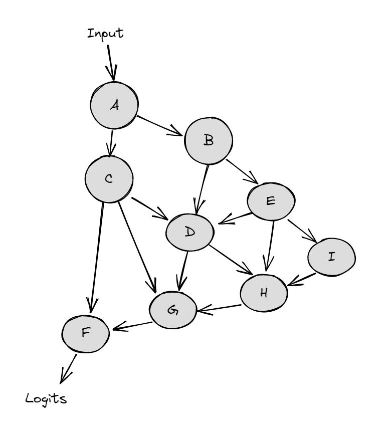
The diagrams below demonstrate activation patching on an abstract neural network (the nodes represent activations, and the arrows between them are weight connections).

A regular forward pass on the clean input looks like:

And activation patching from a corrupted input (green) into a forward pass for the clean input (black) looks like:

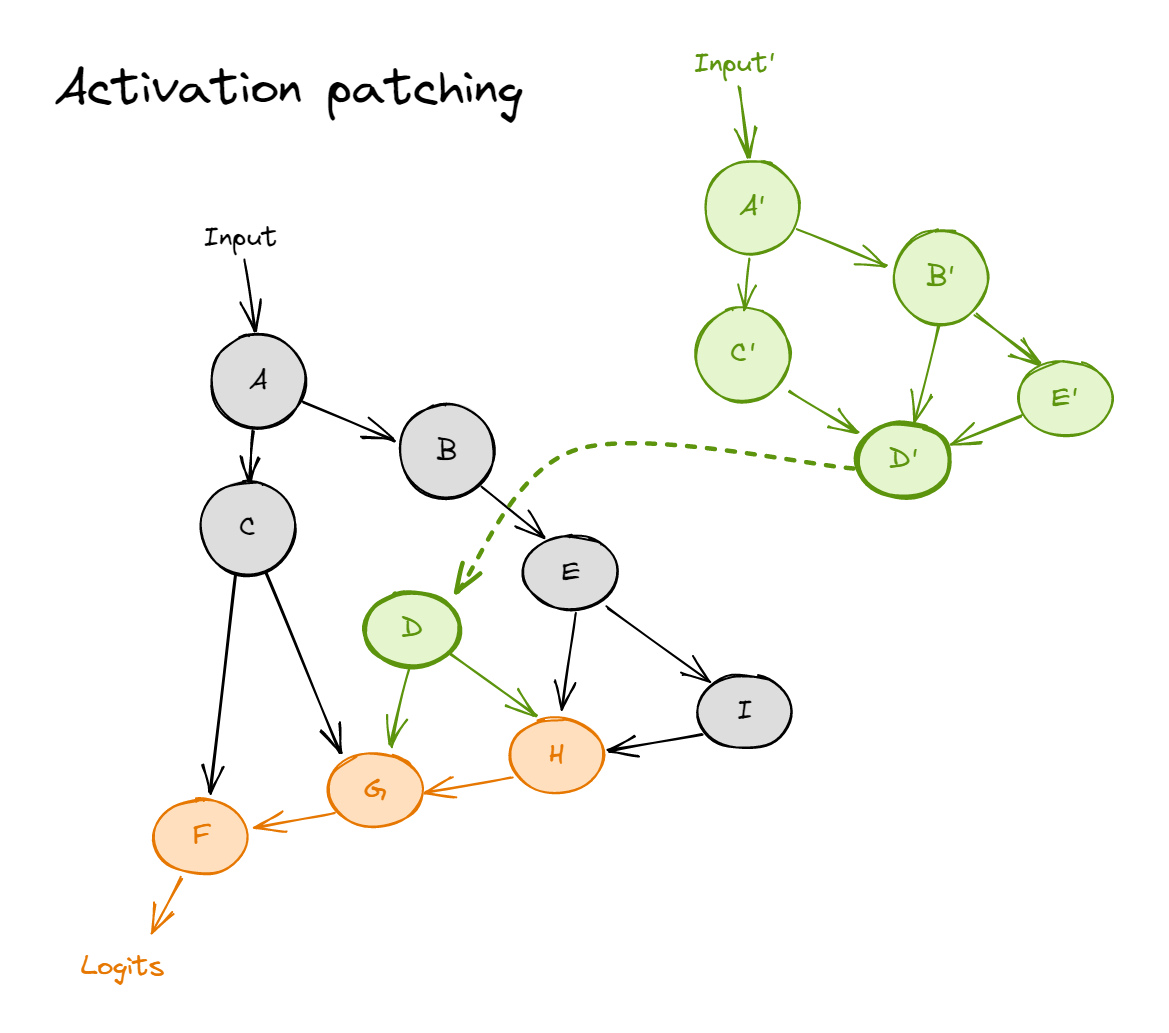
where the dotted line represents patching in a value (i.e. during the forward pass on the clean input, we replace node $D$ with the value it takes on the corrupted input). Nodes $H$, $G$ and $F$ are colored orange, to represent that they now follow a distribution which is not the same as clean or corrupted.

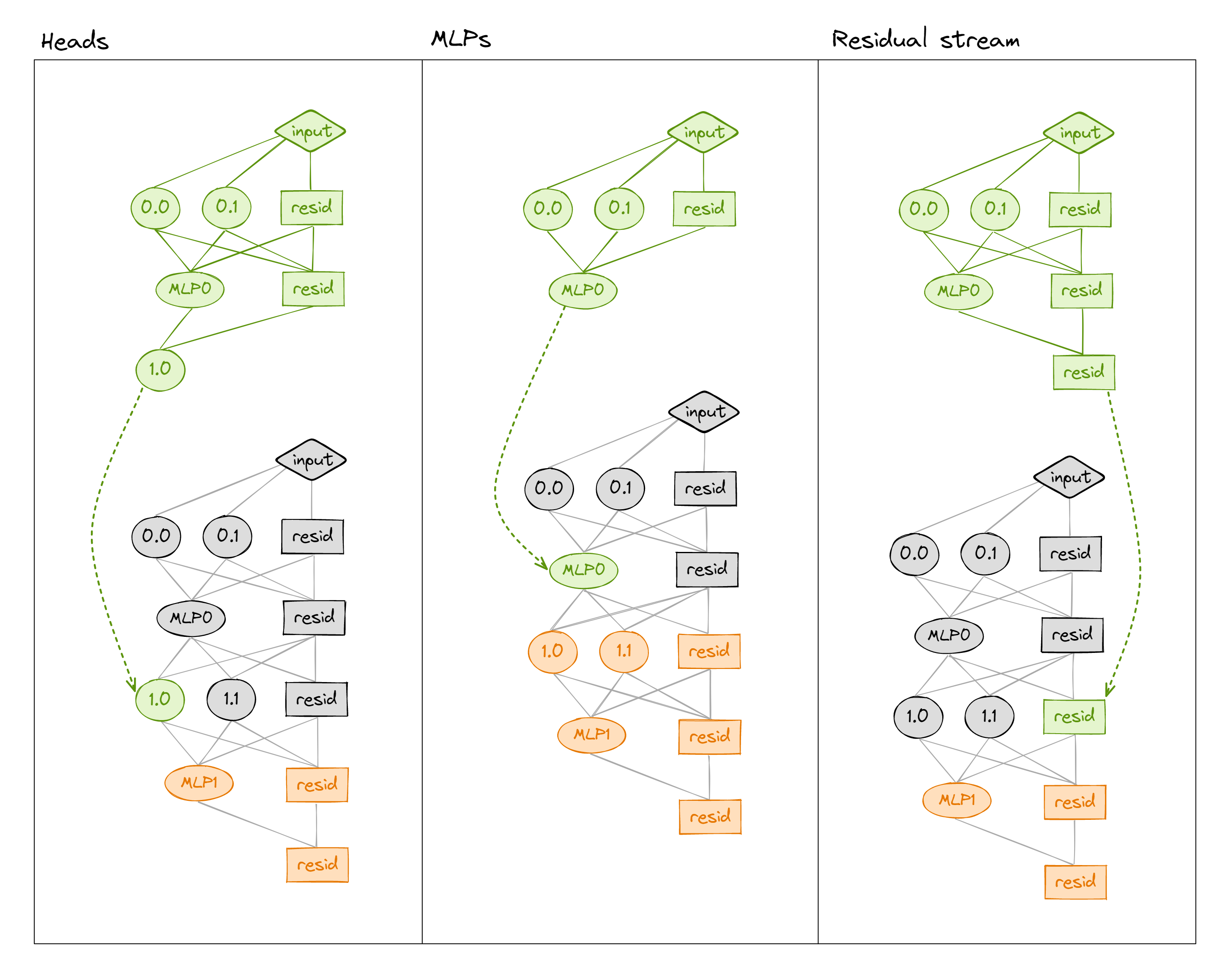
We can patch into a transformer in many different ways (e.g. values of the residual stream, the MLP, or attention heads' output - see below). We can also get even more granular by patching at particular sequence positions (not shown in diagram).

Setting up our patching

Before we patch, we need to decide what our clean and corrupted datasets will be, and create a metric for evaluating a set of logits.

Setting up clean and corrupted moves that result in similar games is non-trivial, so here we take a game and just change the most recent move from E0 to C0. This turns F0 (as a move for white to play) from legal to illegal, so let's make that logit our patching metric.

It also makes sense to have the metric be a linear function of the logit difference. This is enough to uniquely specify a metric.

First, we can plot the original and corrupted boards, to visualize this:

cell_r = 5
cell_c = 4
print(f"Flipping the color of cell {'ABCDEFGH'[cell_r]}{cell_c}")

board = utils.OthelloBoardState()
board.update(focus_games_square[game_index, : move + 1].tolist())
valid_moves = board.get_valid_moves()
flipped_board = copy.deepcopy(board)
flipped_board.state[cell_r, cell_c] *= -1
flipped_legal_moves = flipped_board.get_valid_moves()

newly_legal = [utils.square_to_label(move) for move in flipped_legal_moves if move not in valid_moves]
newly_illegal = [utils.square_to_label(move) for move in valid_moves if move not in flipped_legal_moves]
print("newly_legal", newly_legal)
print("newly_illegal", newly_illegal)

Flipping the color of cell F4
newly_legal []
newly_illegal ['C6']

game_index = 4
move = 20

# Get original & corrupted games (as token IDs & ints)
original_game_id = focus_games_id[game_index, : move + 1]
corrupted_game_id = original_game_id.clone()
corrupted_game_id[-1] = utils.label_to_id("C0")
original_game_square = t.tensor([utils.id_to_square(original_game_id)])
corrupted_game_square = t.tensor([utils.id_to_square(corrupted_game_id)])

original_state, original_legal_moves, original_legal_moves_annotation = get_board_states_and_legal_moves(
    original_game_square
)
corrupted_state, corrupted_legal_moves, corrupted_legal_moves_annotation = get_board_states_and_legal_moves(
    corrupted_game_square
)
utils.plot_board_values(
    t.stack([original_state[move], corrupted_state[move]]),
    text=[original_legal_moves_annotation[move], corrupted_legal_moves_annotation[move]],
    title="Focus game states",
    board_titles=["Original game (black plays E0)", "Corrupted game (black plays C0)"],
    width=650,
    height=380,
)

Next, let's get our logits & cache for both games:

original_logits, original_cache = model.run_with_cache(original_game_id)
corrupted_logits, corrupted_cache = model.run_with_cache(corrupted_game_id)

original_log_probs = original_logits.log_softmax(dim=-1)
corrupted_log_probs = corrupted_logits.log_softmax(dim=-1)

Exercise - create a patching metric

Finally, we'll create a patching metric. This is a function we'll apply to our output logits, in order to measure how much they've changed (in some important way) from their clean values.

We want our patching metric to satisfy the following conditions:

• Should have value one when the logits are the same as in the clean distribution.
• Should have value zero when the logits are the same as in the corrupted distribution.
  • Note - we sometimes use the opposite convention. Either might be justified, depending on the context. Here, you should think of a value of 1 meaning "100% of performance is preserved", and 0 as "performance is gone".
• Should be a linear function of the log probs.
  • Important note - this is not the same as being a linear function of the logits. Can you see why?
• Should just be a function of the logits for the F0 token, at the final game move (since this is the only move that changes between clean and corrupted).
  • Note - you can index into the d_vocab dimension of logits using the f0_index variable defined below.

This should be enough for you to uniquely define your patching metric. Also, note that it should return a scalar tensor (this is important for the transformerlens patching functions to work).

F0_index = utils.label_to_id("F0")
original_F0_log_prob = original_log_probs[0, -1, F0_index]
corrupted_F0_log_prob = corrupted_log_probs[0, -1, F0_index]

print("Check that the model predicts F0 is legal in original game & illegal in corrupted game:")
print(f"Clean log prob: {original_F0_log_prob.item():.2f}")
print(f"Corrupted log prob: {corrupted_F0_log_prob.item():.2f}\n")


def patching_metric(patched_logits: Float[Tensor, "batch seq d_vocab"]) -> Float[Tensor, ""]:
    """
    Function of patched logits, calibrated so that it equals 0 when performance is same as on
    corrupted input, and 1 when performance is same as on original input.

    Should be linear function of the logits for the F0 token at the final move.
    """
    raise NotImplementedError()


tests.test_patching_metric(patching_metric, original_log_probs, corrupted_log_probs)

def patching_metric(patched_logits: Float[Tensor, "batch seq d_vocab"]) -> Float[Tensor, ""]:
    """
    Function of patched logits, calibrated so that it equals 0 when performance is same as on
    corrupted input, and 1 when performance is same as on original input.
    Should be linear function of the logits for the F0 token at the final move.
    """
    patched_log_probs = patched_logits.log_softmax(dim=-1)
    return (patched_log_probs[0, -1, F0_index] - corrupted_F0_log_prob) / (original_F0_log_prob - corrupted_F0_log_prob)

Exercise - write a patching function

Below, you should fill in the functions patch_attn_layer_output and patch_mlp_layer_output.

To do this, you'll have to use TransformerLens hooks. A quick refresher on how they work:

• Hook functions take two compulsory arguments:
  • tensor (a PyTorch tensor of the model's activations at this hookpoint)
  • hook (a HookPoint object, which has helper property hook.name and method hook.layer())
• The function model.run_with_hooks takes arguments:
  • The tokens to run (as first argument)
  • fwd_hooks - a list of (hook_name, hook_fn) tuples. Remember that you can use get_act_name to get hook names.

Tips: - It's good practice to have model.reset_hooks() at the start of functions which add and run hooks. This is because sometimes hooks fail to be removed (if they cause an error while running). There's nothing more frustrating than fixing a hook error only to get the same error message, not realising that you've failed to clear the broken hook! - The HookPoint object has method .layer() and attribute .name which can be useful in your hook functions.

def patch_final_move_output(
    activation: Float[Tensor, "batch seq d_model"],
    hook: HookPoint,
    clean_cache: ActivationCache,
) -> Float[Tensor, "batch seq d_model"]:
    """
    Hook function which patches activations at the final sequence position.

    Note, we only need to patch in the final sequence position, because the prior moves in the clean
    and corrupted input are identical (and this is an autoregressive model).
    """
    raise NotImplementedError()


def get_act_patch_resid_pre(
    model: HookedTransformer,
    corrupted_input: Float[Tensor, "batch pos"],
    clean_cache: ActivationCache,
    patching_metric: Callable[[Float[Tensor, "batch seq d_model"]], Float[Tensor, ""]],
) -> Float[Tensor, "2 n_layers"]:
    """
    Returns an array of results corresponding to the results of patching at each (attn_out, mlp_out)
    for all layers in the model.
    """
    raise NotImplementedError()


patching_results = get_act_patch_resid_pre(model, corrupted_game_id, original_cache, patching_metric)

pd.options.plotting.backend = "plotly"
pd.DataFrame(to_numpy(patching_results.T), columns=["attn", "mlp"]).plot.line(
    title="Layer Output Patching Effect on F0 Log Prob",
    width=700,
    labels={"value": "Patching Effect", "index": "Layer"},
).show()

def patch_final_move_output(
    activation: Float[Tensor, "batch seq d_model"],
    hook: HookPoint,
    clean_cache: ActivationCache,
) -> Float[Tensor, "batch seq d_model"]:
    """
    Hook function which patches activations at the final sequence position.
    Note, we only need to patch in the final sequence position, because the prior moves in the clean
    and corrupted input are identical (and this is an autoregressive model).
    """
    activation[0, -1, :] = clean_cache[hook.name][0, -1, :]
    return activation
def get_act_patch_resid_pre(
    model: HookedTransformer,
    corrupted_input: Float[Tensor, "batch pos"],
    clean_cache: ActivationCache,
    patching_metric: Callable[[Float[Tensor, "batch seq d_model"]], Float[Tensor, ""]],
) -> Float[Tensor, "2 n_layers"]:
    """
    Returns an array of results corresponding to the results of patching at each (attn_out, mlp_out)
    for all layers in the model.
    """
    model.reset_hooks()
    results = t.zeros(2, model.cfg.n_layers, device=device, dtype=t.float32)
    hook_fn = partial(patch_final_move_output, clean_cache=clean_cache)
for i, activation in enumerate(["attn_out", "mlp_out"]):
        for layer in tqdm(range(model.cfg.n_layers)):
            patched_logits = model.run_with_hooks(
                corrupted_input,
                fwd_hooks=[(get_act_name(activation, layer), hook_fn)],
            )
            results[i, layer] = patching_metric(patched_logits)
return results

Recap of this section

We did the following:

• Learned how activation patching worked.
• Constructed the following datasets for patching:
  • Clean distribution = unaltered game,
  • Corrupted distribution = game with a single move flipped (changing th legality of a square),
• Looked at the effect on patching at the output of attention and MLP layers to see which ones changed the output significantly.
  • We found a handful of the MLP layers, and the final attention layer, mattered.
    • Attention layers mostly not mattering was unsurprising, since attention's main job is to move around information rather than operate on it.
  • If we wanted, we could get more granular at this point, and explore which neurons in these layers had a significant effect.