1️⃣ Model Setup & Linear Probes

Learning Objectives

• Understand the basic structure of the Othello-GPT model
• Become familiar with the basic tools we'll use for board visualization during these exercises
• See how our linear probe works, and how we can change basis between "black/white piece" and "mine/their piece"
• Intervene with the linear probe to influence model predictions

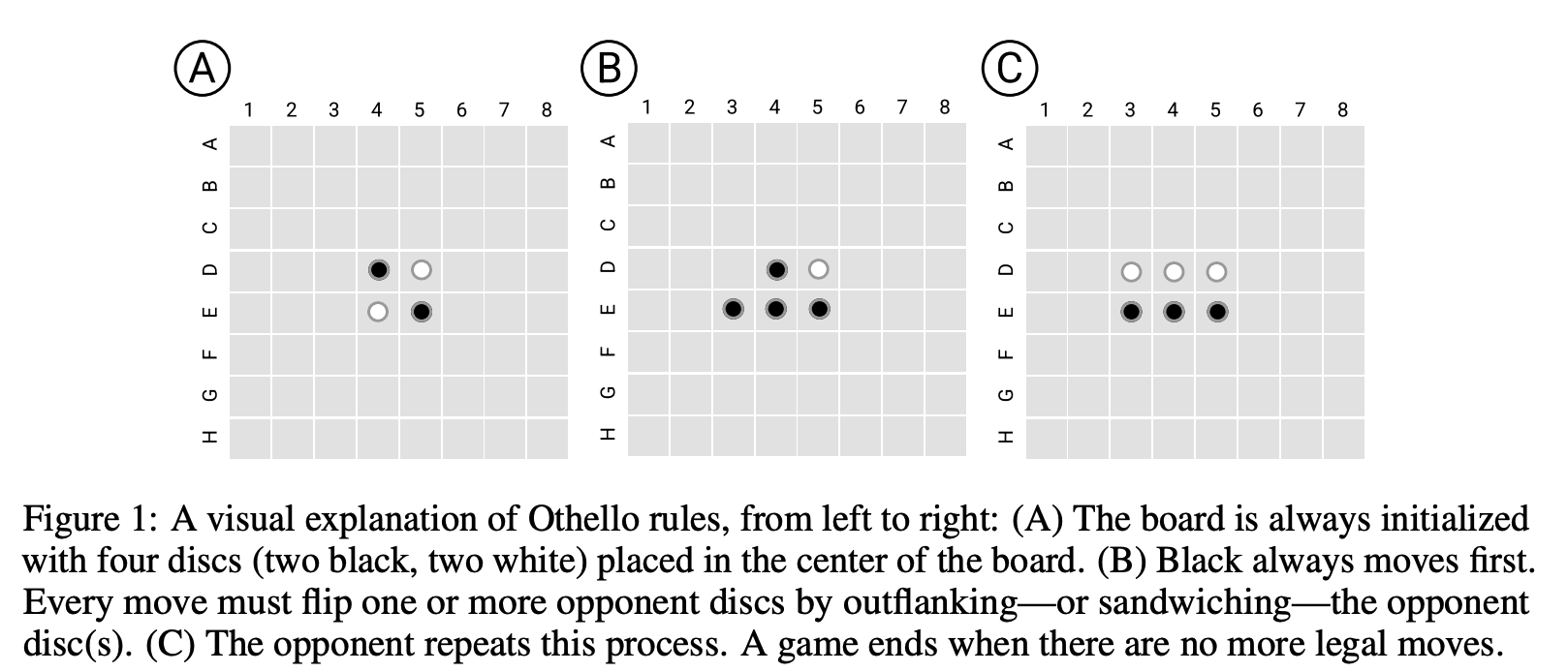
For those unfamiliar, Othello is a board game analogous to chess or go, with two players, black and white, see the rules outlined in the figure below. I found playing the AI on eOthello helpful for building intuition. A single move can change the colour of pieces far away (so long as there's a continuous vertical, horizontal or diagonal line), which means that calculating board state is actually pretty hard! (to my eyes much harder than in chess)

Background - Othello, and OthelloGPT

But despite the model just needing to predict the next move, it spontaneously learned to compute the full board state at each move - a fascinating result. A pretty hot question right now is whether LLMs are just bundles of statistical correlations or have some real understanding and computation! This gives suggestive evidence that simple objectives to predict the next token can create rich emergent structure (at least in the toy setting of Othello). Rather than just learning surface level statistics about the distribution of moves, it learned to model the underlying process that generated that data. In my opinion, it's already pretty obvious that transformers can do something more than statistical correlations and pattern matching, see eg induction heads, but it's great to have clearer evidence of fully-fledged world models!

For context on my investigation, it's worth analysing exactly the two pieces of evidence they had for the emergent world representation, the probes and the causal interventions, and their strengths and weaknesses.

Probes

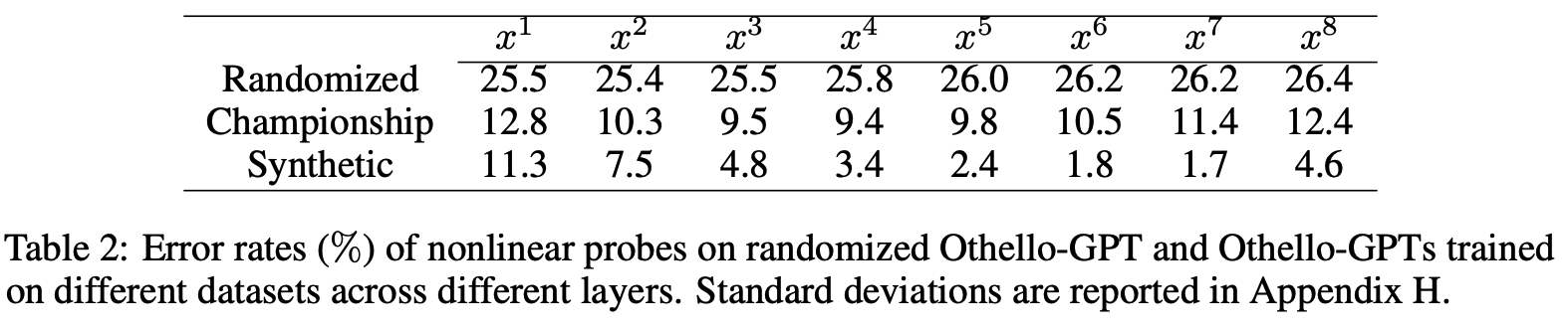
The probes give suggestive, but far from conclusive evidence. When training a probe to extract some feature from a model, it's easy to trick yourself. It's crucial to track whether the probe is just reading out the feature, or actually computing the feature itself, and reading out much simpler features from the model. In the extreme case, you could attach a much more powerful model as your "probe", and have it just extract the input moves, and then compute the board state from scratch! They found that linear probes did not work to recover board state (with an error rate of 20.4%): (ie, projecting the residual stream onto some 3 learned directions for each square, corresponding to empty, black and white logits). While the simplest non-linear probes (a two layer MLP with a single hidden ReLU layer) worked extremely well (an error rate of 1.7%). Further (as described in their table 2, screenshot below), these non-linear probes did not work on a randomly initialised network, and worked better on some layers than others, suggesting they were learning something real from the model.

Causal interventions

Probes on their own can mislead, and don't necessarily tell us that the model uses this representation - the probe could be extracting some vestigial features or a side effect of some more useful computation, and give a misleading picture of how the model computes the solution. But their causal interventions make this much more compelling evidence. They intervene by a fairly convoluted process (detailed in the figure below, though you don't need to understand the details), which boils down to choosing a new board state, and applying gradient descent to the model's residual stream such that our probe thinks the model's residual stream represents the new board state. I have an immediate skepticism of any complex technique like this: when applying a powerful method like gradient descent it's so easy to wildly diverge from what the models original functioning is like! But the fact that the model could do the non-trivial computation of converting an edited board state into a legal move post-edit is a very impressive result! I consider it very strong evidence both that the probe has discovered something real, and that the representation found by the probe is causally linked to the model's actual computation!

Naive Implications for Mechanistic Interpretability

I was very interested in this paper, because it simultaneously had the fascinating finding of an emergent world model (and I'm also generally into any good interp paper), yet something felt off. The techniques used here seemed "too" powerful. The results were strong enough that something here seemed clearly real, but my intuition is that if you've really understood a model's internals, you should just be able to understand and manipulate it with far simpler techniques, like linear probes and interventions, and it's easy to be misled by more powerful techniques.

In particular, my best guess about model internals is that the networks form decomposable, linear representations: that the model computes a bunch of useful features, and represents these as directions in activation space. See Toy Models of Superposition for some excellent exposition on this. This is decomposable because each feature can vary independently (from the perspective of the model - on the data distribution they're likely dependent), and linear because we can extract a feature by projecting onto that feature's direction (if the features are orthogonal - if we have something like superposition it's messier). This is a natural way for models to work - they're fundamentally a series of matrix multiplications with some non-linearities stuck in convenient places, and a decomposable, linear representation allows it to extract any combination of features with a linear map!

Under this framework, if a feature can be found by a linear probe then the model has already computed it, and if that feature is used in a circuit downstream, we should be able to causally intervene with a linear intervention, just changing the coordinate along that feature's direction. So the fascinating finding that linear probes do not work, but non-linear probes do, suggests that either the model has a fundamentally non-linear representation of features (which it is capable of using directly for downstream computation!), or there's a linear representation of simpler and more natural features, from which the probe computes board state. My prior was on a linear representation of simpler features, but the causal intervention findings felt like moderate evidence for the non-linear representation. And the non-linear representation hypothesis would be a big deal if true! If you want to reverse-engineer a model, you need to have a crisp picture of how its computation maps onto activations and weights, and this would break a lot of my beliefs about how this correspondance works! Further, linear representations are just really convenient to reverse-engineer, and this would make me notably more pessimistic about mechanistic interpretability working.

Model Setup & Visualization

The best way to become less confused about a mysterious model behaviour is to mechanistically analyse it. To zoom in on whatever features and circuits we can find, build our understanding from the bottom up, and use this to form grounded beliefs about what's actually going on.

To get started, let's load in the model that we'll be using for this chapter. A few important technical details:

• Othello games have 60 moves (the board has size 8x8, and the middle 4 squares are all occupied, so by 60 moves all squares are occupied by some color). The model's context length is 59, because it's learned to take in moves[0:59] and predict moves[1:60].
• The dataset the model was trained on just consists of randomly sampled legal moves. A move in Othello is legal if and only if it captures the opponents' pieces in a horizontal, vertical or diagonal line - in which case it flips all those pieces to its own color. This means predicting next legal moves is a nontrivial task (one might guess it requires the mdoel to track captures and board states over time)
  • Because the model was trained on cross entropy loss against the actual next moves, the model's distribution converges to uniform over all next legal moves - can you see why?

• The vocabulary size is 61, because we allow any of the 8x8 - 4 = 60 unoccupied squares to be played, plus the pass move. The vocab is ordered pass, A0, A1, ..., H7. Note that we'll be filtering out games where a pass move was played, so we don't need to worry about this.
• We'll refer to squares in 3 different ways:
  1. label - this is the string representation, i.e. "pass", "A0", "A1", ..., "H7".
  2. token id, or id - this is the token ID in the model's vocab, i.e. 1 for A0, ..., 60 for H7. We skip 0 which is the token id for pass, and we skip the 4 middle squares since they're always occupied and so there are no moves in or predictions for these squares.
  3. square index, or square - this is the zero-indexed value of the square in the size-64 board, i.e. 0 for A0, 1 for A1, ..., 63 for H7.
• Black plays first in Othello, and so (in games with no passes) White plays last. Since we don't predict the very first move, this means the model's predictions are for (white 1, black 2, white 2, ..., white 29, black 30, white 30).

Run the code below, to load in the model:

cfg = HookedTransformerConfig(
    n_layers=8,
    d_model=512,
    d_head=64,
    n_heads=8,
    d_mlp=2048,
    d_vocab=61,
    n_ctx=59,
    act_fn="gelu",
    normalization_type="LNPre",
    device=device,
)
model = HookedTransformer(cfg)

state_dict_synthetic = download_file_from_hf("NeelNanda/Othello-GPT-Transformer-Lens", "synthetic_model.pth")
# state_dict_championship = download_file_from_hf("NeelNanda/Othello-GPT-Transformer-Lens", "championship_model.pth")

model.load_state_dict(state_dict_synthetic)

Next, run the code below to check that the model is working correctly. Our sample_input is a sequence of 10 moves (the first 10 moves of the game, starting with black's 1st move and ending in white's 5th move).

# An example input: 10 moves in a game
sample_input = t.tensor([[20, 19, 18, 10, 2, 1, 27, 3, 41, 42]]).to(device)

logits = model(sample_input)
logprobs = logits.log_softmax(-1)

assert logprobs.shape == (1, 10, 61)  # shape is [batch, seq_len, d_vocab]
assert logprobs[0, 0].topk(3).indices.tolist() == [
    21,
    33,
    19,
]  # these are the 3 legal moves, as we'll soon show

Note that we can convert each of our logprob vectors (which have shape (61,)) into a board state tensor of shape (8, 8) (we put very negative values in the 4 middle squares) via some clever indexing. Then, we can plot the results using a helper function utils.plot_board_values we've written for you. Since you'll be using this function a lot in subsequent exercises, we'll go through the important arguments here:

• state: a tensor of shape (*N, 8, 8), where *N is any number of batch dimensions. For each N tensors, we'll visualize a single 8x8 grid. If the shape is (8, 8) then we'll plot a single board.
• board_titles: if plotting multiple boards (i.e. N > 1) then we can use this argument to label each of them.
• boards_per_row: if plotting multiple boards, we can set this many boards per row.
• text: an optional list of strings with the same shape as state, which we can use to annotate the boards. Also fine for it to be broadcastable to the shape of state (e.g. it can be (8, 8) even if state is 3D).
• kwargs: other arguments get passed into px.imshow (e.g. title, width and height)

Understanding exactly how this function works isn't important, since you can always copy and paste code from one of the following examples if you forget how to use it!

MIDDLE_SQUARES = [27, 28, 35, 36]
ALL_SQUARES = [i for i in range(64) if i not in MIDDLE_SQUARES]

logprobs_board = t.full(size=(8, 8), fill_value=-13.0, device=device)
logprobs_board.flatten()[ALL_SQUARES] = logprobs[0, 0, 1:]  # the [1:] is to filter out logits for the "pass" move

utils.plot_board_values(logprobs_board, title="Example Log Probs", width=500)

We can use the text argument to annotate all the legal squares with their token IDs, which might be easier in some cases. Here's an example (you might want to reuse this code in some later exercises):

TOKEN_IDS_2D = np.array([str(i) if i in ALL_SQUARES else "" for i in range(64)]).reshape(8, 8)
BOARD_LABELS_2D = np.array(["ABCDEFGH"[i // 8] + f"{i % 8}" for i in range(64)]).reshape(8, 8)

print(TOKEN_IDS_2D)
print(BOARD_LABELS_2D)

utils.plot_board_values(
    t.stack([logprobs_board, logprobs_board]),  # shape (2, 8, 8)
    title="Example Log Probs (with annotated token IDs)",
    width=800,
    text=np.stack([TOKEN_IDS_2D, BOARD_LABELS_2D]),  # shape (2, 8, 8)
    board_titles=["Labelled by token ID", "Labelled by board label"],
)

[['0' '1' '2' '3' '4' '5' '6' '7']
 ['8' '9' '10' '11' '12' '13' '14' '15']
 ['16' '17' '18' '19' '20' '21' '22' '23']
 ['24' '25' '26' '' '' '29' '30' '31']
 ['32' '33' '34' '' '' '37' '38' '39']
 ['40' '41' '42' '43' '44' '45' '46' '47']
 ['48' '49' '50' '51' '52' '53' '54' '55']
 ['56' '57' '58' '59' '60' '61' '62' '63']]
[['A0' 'A1' 'A2' 'A3' 'A4' 'A5' 'A6' 'A7']
 ['B0' 'B1' 'B2' 'B3' 'B4' 'B5' 'B6' 'B7']
 ['C0' 'C1' 'C2' 'C3' 'C4' 'C5' 'C6' 'C7']
 ['D0' 'D1' 'D2' 'D3' 'D4' 'D5' 'D6' 'D7']
 ['E0' 'E1' 'E2' 'E3' 'E4' 'E5' 'E6' 'E7']
 ['F0' 'F1' 'F2' 'F3' 'F4' 'F5' 'F6' 'F7']
 ['G0' 'G1' 'G2' 'G3' 'G4' 'G5' 'G6' 'G7']
 ['H0' 'H1' 'H2' 'H3' 'H4' 'H5' 'H6' 'H7']]

We can also use this function to plot multiple board states at once, exactly the same way. Again pay attention to the indexing, because understanding how this works will be useful going forwards!

logprobs_multi_board = t.full(size=(10, 8, 8), fill_value=-13.0, device=device)
logprobs_multi_board.flatten(1, -1)[:, ALL_SQUARES] = logprobs[0, :, 1:]  # we now do all 10 moves at once

utils.plot_board_values(
    logprobs_multi_board,
    title="Example Log Probs",
    width=1000,
    boards_per_row=5,
    board_titles=[f"Logprobs after move {i}" for i in range(1, 11)],
)

Let's use the same function to plot the first 10 board states, and check that the predictions shown above make sense given the board state at that time. We'll use a helper method OthelloBoardState to track the board state after each move.

board_states = t.zeros((10, 8, 8), dtype=t.int32)
legal_moves = t.zeros((10, 8, 8), dtype=t.int32)

board = utils.OthelloBoardState()
for i, token_id in enumerate(sample_input.squeeze()):
    # board.umpire takes a square index (i.e. from 0 to 63) and makes a move on the board
    board.umpire(utils.id_to_square(token_id))

    # board.state gives us the 8x8 numpy array of 0 (blank), -1 (black), 1 (white)
    board_states[i] = t.from_numpy(board.state)

    # board.get_valid_moves() gives us a list of the indices of squares that are legal to play next
    legal_moves[i].flatten()[board.get_valid_moves()] = 1

# Turn `legal_moves` into strings, with "o" where the move is legal and empty string where illegal
legal_moves_annotation = np.where(to_numpy(legal_moves), "o", "").tolist()

utils.plot_board_values(
    board_states,
    title="Board states",
    width=1000,
    boards_per_row=5,
    board_titles=[f"State after move {i}" for i in range(1, 11)],
    text=legal_moves_annotation,
)

In this plot you should see that each board state evolves from the previous one via a single move that captures a set of pieces from the opposing color (e.g. in the first move black plays C3 capturing white at D3, and in the second move white plays C2 and captures back black diagonally at D3). You should also see that the annotated legal moves match the moves predicted by the model.

Data

Let's now load some data for OthelloGPT. We'll load data in in id format (i.e. 1 to 60 inclusive, since our vocab is range(0, 61) and we're filtering out games with pass moves) and int format (i.e. 0 to 63 inclusive, since the games contain moves from A0 to H7).

board_seqs_id = t.from_numpy(np.load(section_dir / "board_seqs_id_small.npy")).long()
board_seqs_square = t.from_numpy(np.load(section_dir / "board_seqs_square_small.npy")).long()

print(f"board_seqs_id: shape {tuple(board_seqs_id.shape)}, range: {board_seqs_id.min()} to {board_seqs_id.max()}")
print(
    f"board_seqs_square: shape {tuple(board_seqs_square.shape)}, range: {board_seqs_square.min()} to {board_seqs_square.max()}"
)

board_seqs_id: shape (100000, 60), range: 1 to 60
board_seqs_square: shape (100000, 60), range: 0 to 63

Note - you can access a larger dataset at the GitHub readme, in the "Training Othello-GPT" section. There are links to download datasets from Google Drive (both synthetic and championship games). You can store them in your data folder, after you've cloned the repo using the code above.

Making some utilities

At this point, we'll stop and get some aggregate data that will be useful later - a tensor of valid moves, of board states, and a cache of all model activations across 50 games (in practice, you want as much as will comfortably fit into GPU memory). It's really convenient to have the ability to quickly run an experiment across a bunch of games! And one of the great things about small models on algorithmic tasks is that you just can do stuff like this.

Let's call these the focus games.

def get_board_states_and_legal_moves(
    games_square: Int[Tensor, "n_games n_moves"],
) -> tuple[
    Int[Tensor, "n_games n_moves rows cols"],
    Int[Tensor, "n_games n_moves rows cols"],
    list,
]:
    """
    Returns the following:
        states:                 (n_games, n_moves, 8, 8): tensor of board states after each move
        legal_moves:            (n_games, n_moves, 8, 8): tensor of 1s for legal moves, 0s for
                                    illegal moves
        legal_moves_annotation: (n_games, n_moves, 8, 8): list containing strings of "o" for legal
                                    moves (for plotting)
    """
    # Create tensors to store the board state & legal moves
    n_games, n_moves = games_square.shape
    states = t.zeros((n_games, 60, 8, 8), dtype=t.int32)
    legal_moves = t.zeros((n_games, 60, 8, 8), dtype=t.int32)

    # Loop over each game, populating state & legal moves tensors after each move
    for n in range(n_games):
        board = utils.OthelloBoardState()
        for i in range(n_moves):
            board.umpire(games_square[n, i].item())
            states[n, i] = t.from_numpy(board.state)
            legal_moves[n, i].flatten()[board.get_valid_moves()] = 1

    # Convert legal moves to annotation
    legal_moves_annotation = np.where(to_numpy(legal_moves), "o", "").tolist()

    return states, legal_moves, legal_moves_annotation


num_games = 50

focus_games_id = board_seqs_id[:num_games]  # shape [50, 60]
focus_games_square = board_seqs_square[:num_games]  # shape [50, 60]
focus_states, focus_legal_moves, focus_legal_moves_annotation = get_board_states_and_legal_moves(focus_games_square)

print("focus states:", focus_states.shape)
print("focus_legal_moves", tuple(focus_legal_moves.shape))

# Plot the first 10 moves of the first game
utils.plot_board_values(
    focus_states[0, :10],
    title="Board states",
    width=1000,
    boards_per_row=5,
    board_titles=[f"Move {i}, {'white' if i % 2 == 1 else 'black'} to play" for i in range(1, 11)],
    text=np.where(to_numpy(focus_legal_moves[0, :10]), "o", "").tolist(),
)

focus states: torch.Size([50, 60, 8, 8])
focus_legal_moves (50, 60, 8, 8)

Let's also cache all the model's activations and logits for these focus games.

focus_logits, focus_cache = model.run_with_cache(focus_games_id[:, :-1].to(device))

print(focus_logits.shape)  # shape [num_games=50, n_ctx=59, d_vocab=61]

torch.Size([50, 59, 61])

Recap of the useful objects we've defined

We have the following:

Models - model is an 8-layer autoregressive transformer, trained to predict legal Othello moves. Its vocab is range(0, 61) where 0 = "pass" and the other numbers represent the 60 possible moves, excluding the 4 middle squares

All data - board_seqs_id, shape (100k, 60) contains the moves from all 100k games (as token ids) - board_seqs_square, shape (100k, 60) contains the moves from all 100k games (as ints)

Focus games data - focus_games_id, shape (50, 60) contains the moves from 50 games (as token ids) - focus_games_square, shape (50, 60) contains the moves from 50 games (as ints) - focus_states, shape (50, 60, 8, 8) contains the board states after each move (0 = empty, 1 = black, -1 = white) - focus_legal_moves, shape (50, 60, 8, 8) contains a 1 for each legal move, and 0 for each illegal move - focus_logits, shape (50, 59, 61) contains model's output logits on focus games - 59=model.cfg.n_ctx because we don't include the final move in our forward pass, and 61=model.cfg.d_vocab contains the "pass" move and all 60 playable squares

What is a probe?

From the MI Dynalist notes:

Probing is a technique for identifying directions in network activation space that correspond to a concept/feature.

In spirit, you give the network a bunch of inputs with that feature, and a bunch without it. You train a linear map on a specific activation (eg the output of layer 5) which distinguishes these two sets, giving a 1D linear map (a probe), corresponding to a direction in activation space, which likely corresponds to that feature.

Probes can be a very valuable tool to help us better understand the concepts represented in our model. However, there are two big caveats to keep in mind:

1. Probes give us a direction, but they don't give us a causal story about how that direction got into the model in the first place, or how the model is using that direction.
2. Probes (especially nonlinear probes) can be hiding a lot of computation under their surface.

In the original paper analysing Othello, the authors used nonlinear probing to find important directions. This went against a fundamental intuition - that models fundamentally store things in linear ways, and so we should be able to access them with linear probes. In these exercises, we'll be using linear probes.

Using the probe

The training of this probe was kind of a mess, and I'd do a bunch of things differently if doing it again.

There were 3 different probe modes:

• full_linear_probe[0].shape = (d_model, 8, 8, 3) was trained on black to play, i.e. odd moves. The classes are [empty, white, black].
• full_linear_probe[1].shape = (d_model, 8, 8, 3) was trained on white to play, i.e. even moves. The classes are [empty, white, black].
• full_linear_probe[2].shape = (d_model, 8, 8, 3) was trained on all moves.

For example, we could take full_linear_probe[0] and take the inner product with the residual stream to get a tensor of shape (8, 8, 3) representing 8x8=64 separate predictions for what each of the 64 board squares contains (i.e. you'd softmax this tensor over the last dimension to get probabilities).

full_linear_probe = t.load(section_dir / "main_linear_probe.pth", map_location=str(device), weights_only=True)

print(full_linear_probe.shape)

# Define indices along `full_linear_probe.shape[0]`, i.e. the different probe modes
black_to_play, white_to_play, _ = (0, 1, 2)
# Define indices along `full_linear_probe.shape[-1]`, i.e. the different classifications for each mode
empty, white, black = (0, 1, 2)

torch.Size([3, 512, 8, 8, 3])

Exercise - calculate probe cosine similarities

We won't be using full_linear_probe[2] much, since it doesn't work very well. We'll be focusing on the first two modes.

The key result that was found in this investigation is that the probe learns directions in terms of "theirs vs mine" rather than "black vs white". In this case, you'd expect the probes for odd and even moves to be approximately opposite to each other (since "theirs vs mine" has the opposite meaning in odd vs even moves). Here's a plot visualizing that we do in fact get this - it shows the cosine similarity of the "black minus white" directions across each 64 squares in each of the probe modes. The off diagonal stripe with values close to negative 1 indicates that the "black minus white" direction for any given square is approximately antipodal when taken at odd vs even modes (marked with (O) and (E) in the reference plot).

Try to replicate this plot, using just the full_linear_probe that's been defined for you above. Remember, it has shape (modes=3, d_model=512, rows=8, cols=8, options=3): the first 2 modes are black to play / white to play, and the three options are empty / white / black. We've given you the code to create the plot from the cosine_similarities tensor (which should have shape (64*2, 64*2)), all you need to do is create the tensor.

# YOUR CODE HERE - define `cosine_similarities`, then run the cell to create the plot

fig = px.imshow(
    to_numpy(cosine_similarities),
    title="Cosine Sim of B-W Linear Probe Directions by Cell",
    x=[f"{label} (O)" for label in BOARD_LABELS_2D.flatten()] + [f"{label} (E)" for label in BOARD_LABELS_2D.flatten()],
    y=[f"{label} (O)" for label in BOARD_LABELS_2D.flatten()] + [f"{label} (E)" for label in BOARD_LABELS_2D.flatten()],
    width=900,
    height=800,
    color_continuous_scale="RdBu",
    color_continuous_midpoint=0.0,
)
fig.show()

# Get the "black vs white" probe directions for odd & even moves respectively
black_vs_white_dir_odd_moves = (
    full_linear_probe[black_to_play, :, :, :, black] - full_linear_probe[black_to_play, :, :, :, white]
)
black_vs_white_dir_even_moves = (
    full_linear_probe[white_to_play, :, :, :, black] - full_linear_probe[white_to_play, :, :, :, white]
)
# Flatten over (rows, cols) then concatenate them over this dimension
all_dirs = t.stack([black_vs_white_dir_odd_moves, black_vs_white_dir_even_moves])
all_dirs = einops.rearrange(all_dirs, "parity d_model rows cols -> d_model (parity rows cols)")
# Compute cosine similarities
all_dirs_normed = all_dirs / all_dirs.norm(dim=0, keepdim=True)
cosine_similarities = einops.einsum(
    all_dirs_normed,
    all_dirs_normed,
    "d_model mode_row_col_1, d_model mode_row_col_2 -> mode_row_col_1 mode_row_col_2",
)

Changing probe basis

Now we've established that the probe directions are very similar, let's just average them to create our probe in a new basis: the "theirs vs mine" basis, not the "black vs white" basis. For example, our new probe's "theirs" direction will be the average of the white direction when black is to play, and the black direction when white is to play.

linear_probe = t.stack(
    [
        # "Empty" direction = average of empty direction across probe modes
        full_linear_probe[[black_to_play, white_to_play], ..., [empty, empty]].mean(0),
        # "Theirs" direction = average of {x to play, classification != x} across probe modes
        full_linear_probe[[black_to_play, white_to_play], ..., [white, black]].mean(0),
        # "Mine" direction = average of {x to play, classification == x} across probe modes
        full_linear_probe[[black_to_play, white_to_play], ..., [black, white]].mean(0),
    ],
    dim=-1,
)

Let's test out our new probe, by applying it to move 29 in game 0 from our focus games. This is an odd move, so black is to play.

def plot_probe_outputs(
    cache: ActivationCache,
    linear_probe: Tensor,
    layer: int,
    game_index: int,
    move: int,
    title: str = "Probe outputs",
):
    residual_stream = cache["resid_post", layer][game_index, move]
    probe_out = einops.einsum(residual_stream, linear_probe, "d_model, d_model row col options -> options row col")

    utils.plot_board_values(
        probe_out.softmax(dim=0),
        title=title,
        width=900,
        height=400,
        board_titles=["P(Empty)", "P(Their's)", "P(Mine)"],
        # text=BOARD_LABELS_2D,
    )


layer = 6
game_index = 0
move = 29

utils.plot_board_values(
    focus_states[game_index, move],
    title="Focus game states",
    width=400,
    height=400,
    text=focus_legal_moves_annotation[game_index][move],
)

plot_probe_outputs(
    focus_cache,
    linear_probe,
    layer,
    game_index,
    move,
    title="Probe outputs after move 29 (black to play)",
)

Moving back to layer 3, it seems the model already has a pretty good board state representation by this point, but it's missing a few things (most notably it thinks C5 and especially C6 are white when they're actually black). My guess is that the board state calculation circuits haven't quite finished and are doing some iterative reasoning - if those cells have been taken several times, maybe it needs a layer to track the next earliest time it was taken? I don't know, and figuring this out would be a great starter project if you want to explore!

layer = 3
game_index = 0
move = 29

plot_probe_outputs(
    focus_cache,
    linear_probe,
    layer,
    game_index,
    move,
    title="Probe outputs (layer 4) after move 29 (black to play)",
)

Now let's take one step forward - we should see that the representations totally flip. This is indeed what we find.

layer = 4
game_index = 0
move = 30

utils.plot_board_values(
    focus_states[game_index, move],
    text=focus_legal_moves_annotation[game_index][move],
    title="Focus game states",
    width=400,
    height=400,
)
plot_probe_outputs(
    focus_cache,
    linear_probe,
    layer,
    game_index,
    move,
    title="Probe outputs (layer 4) after move 30 (white to play)",
)

Notice that the model gets the corner wrong in this case (incorrectly thinking that the corner is white rather than empty) - it's not a big deal, but interesting!

Can you think of a reason why corners might be treated differently in this model?

Computing accuracy

Hopefully I've convinced you anecdotally that a linear probe works. But to be more rigorous, let's check accuracy across our 50 games.

# Create a tensor of "their vs mine" board states (by flipping even parities of the "focus_states" tensor)
focus_states_theirs_vs_mine = focus_states * (-1 + 2 * (t.arange(focus_states.shape[1]) % 2))[None, :, None, None]

# Convert values (0: empty, 1: theirs, -1: mine) to (0: empty, 1: theirs, 2: mine)
focus_states_theirs_vs_mine[focus_states_theirs_vs_mine == 1] = 2
focus_states_theirs_vs_mine[focus_states_theirs_vs_mine == -1] = 1

# Get probe values at layer 6, and compute the probe predictions
probe_out = einops.einsum(
    focus_cache["resid_post", 6],
    linear_probe,
    "game move d_model, d_model row col options -> game move row col options",
)
probe_predictions = probe_out.argmax(dim=-1)

# Get accuracy at odd, even & all moves (average over games & moves)
correct_middle_odd_answers = (probe_predictions.cpu() == focus_states_theirs_vs_mine[:, :-1])[:, 5:-5:2]
accuracies_odd = einops.reduce(correct_middle_odd_answers.float(), "game move row col -> row col", "mean")

correct_middle_even_answers = (probe_predictions.cpu() == focus_states_theirs_vs_mine[:, :-1])[:, 6:-5:2]
accuracies_even = einops.reduce(correct_middle_even_answers.float(), "game move row col -> row col", "mean")

correct_middle_answers = (probe_predictions.cpu() == focus_states_theirs_vs_mine[:, :-1])[:, 5:-5]
accuracies = einops.reduce(correct_middle_answers.float(), "game move row col -> row col", "mean")

# Plot accuracies
utils.plot_board_values(
    1 - t.stack([accuracies_odd, accuracies_even, accuracies], dim=0),
    title="Average Error Rate of Linear Probe",
    width=1000,
    height=400,
    board_titles=["Black to play", "White to play", "All moves"],
    zmax=0.25,
    zmin=-0.25,
)

Note that we can see the probe is worse near corners, as we anecdotally observed.

Intervening with the probe

One of the really exciting consequences of a linear probe is that it gives us a set of interpretable directions in the residual stream! And with this, we can not only interpret the model's representations, but we can also intervene in the model's reasoning. This is a good proof of concept that if you can really understand a model, you can get precise and detailed control over its behaviour.

The first step is to convert our probe to meaningful directions. Each square's probe has 3 vectors, but the logits go into a softmax, which is translation invariant, so this only has two degrees of freedom. A natural-ish way to convert it into two vectors is taking blank - (mine + theirs)/2 giving a "is this cell empty or not" direction and mine - theirs giving a "conditional on being blank, is this my colour vs their's" direction.

Having a single meaningful direction is important, because it allows us to interpret a feature or intervene on it. The original three directions has one degree of freedom, so each direction is arbitrary on its own.

Exercise - define your probe directions

Define the tensors blank_probe and my_prob, which point in the two directions given above.

# YOUR CODE HERE - define `blank_probe` and `my_probe`, from linear combinations of `linear_probe`

tests.test_my_probes(blank_probe, my_probe, linear_probe)

# blank(0) - (theirs(1) + mine(2))/2
blank_probe = linear_probe[..., 0] - linear_probe[..., 1]  0.5 - linear_probe[..., 2]  0.5
# mine(2) - theirs(1)
my_probe = linear_probe[..., 2] - linear_probe[..., 1]

Now that we've got our probe working, let's see it in action!

We'll take the 20th move in the 0th game as our example:

game_index = 0
move = 20

# Plot board state
utils.plot_board_values(
    focus_states[game_index, move],
    title="Focus game states",
    width=400,
    height=400,
    text=focus_legal_moves_annotation[game_index][move],
)

# Plot model predictions
logprobs = t.full(size=(8, 8), fill_value=-13.0, device=device)
logprobs.flatten()[ALL_SQUARES] = focus_logits[game_index, move].log_softmax(dim=-1)[1:]
utils.plot_board_values(logprobs, title=f"Logprobs after move {move}", width=450, height=400)

Now, how does the game state (i.e. which moves are legal for white) change when F4 is flipped from black to white?

Let's verify this, using the OthelloBoardState class:

cell_r = 5
cell_c = 4
print(f"Flipping the color of cell {'ABCDEFGH'[cell_r]}{cell_c}")

board = utils.OthelloBoardState()
board.update(focus_games_square[game_index, : move + 1].tolist())
valid_moves = board.get_valid_moves()
flipped_board = copy.deepcopy(board)
flipped_board.state[cell_r, cell_c] *= -1
flipped_legal_moves = flipped_board.get_valid_moves()

newly_legal = [utils.square_to_label(move) for move in flipped_legal_moves if move not in valid_moves]
newly_illegal = [utils.square_to_label(move) for move in valid_moves if move not in flipped_legal_moves]
print("newly_legal", newly_legal)
print("newly_illegal", newly_illegal)

Flipping the color of cell F4
newly_legal ['D2']
newly_illegal ['G4']

We can now intervene on the model's residual stream using the "my colour vs their colour" direction. I get the best results intervening after layer 4. This is a linear intervention - we are just changing a single dimension of the residual stream and keeping the others unchanged. This is a fairly simple intervention, and it's striking that it works!

I apply the fairly janky technique of taking current coordinate in the given direction, negating it, and then multiply by a hyperparameter called scale (scale between 1 and 8 tends to work best - small isn't enough and big tends to break things). I haven't tried hard to optimise this and I'm sure it can be improved! Eg by replacing the model's coordinate by a constant rather than scaling it. I also haven't dug into the best scale parameters, or which ones work best in which contexts - plausibly different cells have different activation scales on their world models and need different behaviour!

Exercise - define the apply_scale function

Define a function which will take in the residual stream value and the associated hook point as arguments, and return a modified version of the residual stream, in the way described above.

To be clear, if we define $\vec{v}$ as the probe's flip direction for a given square (called flip_dir below), then we can write our residual stream (at pos=20, which is the one we're interested in) as the vector:

where $\vec{w}$ is some vector orthogonal to $v$. We want to alter the residual stream at this position to be:

Remember to normalize vector $\vec{v}$!

def apply_scale(
    resid: Float[Tensor, "batch seq d_model"],
    flip_dir: Float[Tensor, "d_model"],
    scale: int,
    pos: int,
) -> Float[Tensor, "batch seq d_model"]:
    """
    Returns a version of the residual stream, modified by the amount `scale` in the
    direction `flip_dir` at the sequence position `pos`, in the way described above.
    """
    raise NotImplementedError()


tests.test_apply_scale(apply_scale)

def apply_scale(
    resid: Float[Tensor, "batch seq d_model"],
    flip_dir: Float[Tensor, "d_model"],
    scale: int,
    pos: int,
) -> Float[Tensor, "batch seq d_model"]:
    """
    Returns a version of the residual stream, modified by the amount scale in the
    direction flip_dir at the sequence position pos, in the way described above.
    """
    flip_dir_normed = flip_dir / flip_dir.norm()
alpha = resid[0, pos] @ flip_dir_normed
    resid[0, pos] -= (scale + 1)  alpha  flip_dir_normed
return resid

Now, you can run the code below to see the output of your interventions. You should see that the model's prediction changes, it starts predicting D2 as legal and G4 as illegal.

flip_dir = my_probe[:, cell_r, cell_c]

logprobs_flipped = []
layer = 4
scales = [0, 1, 2, 4, 8, 16]

# Iterate through scales, generate a new facet plot for each possible scale
for scale in scales:
    # Hook function which will perform flipping in the "F4 flip direction"
    def flip_hook(resid: Float[Tensor, "batch seq d_model"], hook: HookPoint):
        return apply_scale(resid, flip_dir, scale, move)

    # Calculate the logits for the board state, with the `flip_hook` intervention (note that we only
    # need to use :move+1 as input, because of causal attention)
    flipped_logits = model.run_with_hooks(
        focus_games_id[game_index : game_index + 1, : move + 1],
        fwd_hooks=[
            (get_act_name("resid_post", layer), flip_hook),
        ],
    ).log_softmax(dim=-1)[0, move]

    logprobs_flipped_single = t.zeros((64,), dtype=t.float32, device=device) - 10.0
    logprobs_flipped_single[ALL_SQUARES] = flipped_logits.log_softmax(dim=-1)[1:]
    logprobs_flipped.append(logprobs_flipped_single)

flip_state_big = t.stack(logprobs_flipped)
logprobs_repeated = einops.repeat(logprobs.flatten(), "d -> b d", b=6)
color = t.zeros((len(scales), 64)) + 0.2
color[:, utils.to_square(newly_legal)] = 1
color[:, utils.to_square(newly_illegal)] = -1

scatter(
    y=logprobs_repeated,
    x=flip_state_big,
    title=f"Original vs Flipped {utils.square_to_label(8 * cell_r + cell_c)} at Layer {layer}",
    xaxis="Flipped",
    yaxis="Original",
    hover=[f"{r}{c}" for r in "ABCDEFGH" for c in range(8)],
    facet_col=0,
    facet_labels=[f"Translate by {i}x" for i in scales],
    color=color,
    color_name="Newly Legal",
    color_continuous_scale="Geyser",
    width=1400,
)

Final recap of the useful objects we've defined

We have the following:

Models - model is an 8-layer autoregressive transformer, trained to predict legal Othello moves. Its vocab is range(0, 61) where 0 = "pass" and the other numbers represent the 60 possible moves, excluding the 4 middle squares - full_linear_probe.shape = (mode=3, d_model=512, row=8, col=8, options=3), probe in the "black/white basis" (modes are black/white/both to play, options are empty/white/black) - linear_probe.shape = (d_model=512, row=8, col=8, options=3), probe in the "theirs/mine basis" (options are empty/theirs/mine) - blank_probe and my_probe, both have shape (d_model=512, row=8, col=8) and are created from linear combinations of the linear_probe options

All data - board_seqs_id.shape = (100k, 60) contains the moves from all 100k games (as token ids) - board_seqs_square.shape = (100k, 60) contains the moves from all 100k games (as ints)

Focus games data - focus_games_id.shape = (50, 60) contains the moves from 50 games (as token ids) - focus_games_square.shape = (50, 60) contains the moves from 50 games (as ints) - focus_states.shape = (50, 60, 8, 8) contains the board states after each move (0 = empty, 1 = black, -1 = white) - focus_legal_moves.shape = (50, 60, 8, 8) contains a 1 for each legal move, and 0 for each illegal move - focus_logits.shape = (50, 59, 61) contains model's output logits on focus games (59 because we don't include the final move in our fwd pass, 61 because our vocab size is 61 - we have 60 moves + 1 for pass)