[1.5.2] Grokking and Modular Arithmetic
Please send any problems / bugs on the #errata channel in the Slack group, and ask any questions on the dedicated channels for this chapter of material.
If you want to change to dark mode, you can do this by clicking the three horizontal lines in the top-right, then navigating to Settings → Theme.
Links to all other chapters: (0) Fundamentals, (1) Transformer Interpretability, (2) RL.
Note - if you get a numpy-related error at any point (possibly
module 'numpy.linalg._umath_linalg' has no attribute '_ilp64'), you should restart the kernel and run the setup code again. The error should go away.

Introduction
Our goal for today is to reverse-engineer a one-layer transformer trained on modular addition! It turns out that the circuit responsible for this involves discrete Fourier transforms and trigonometric identities. This is perhaps the most interesting circuit for solving an algorithmic task that has been fully reverse-engineered thus far.
These exercises are adapted from the original notebook by Neel Nanda and Tom Lierberum (and to a lesser extent the accompanying paper). We'll mainly be focusing on mechanistic analysis of this toy model, rather than replicating the grokking results (these may come in later exercises).
Problem Setup
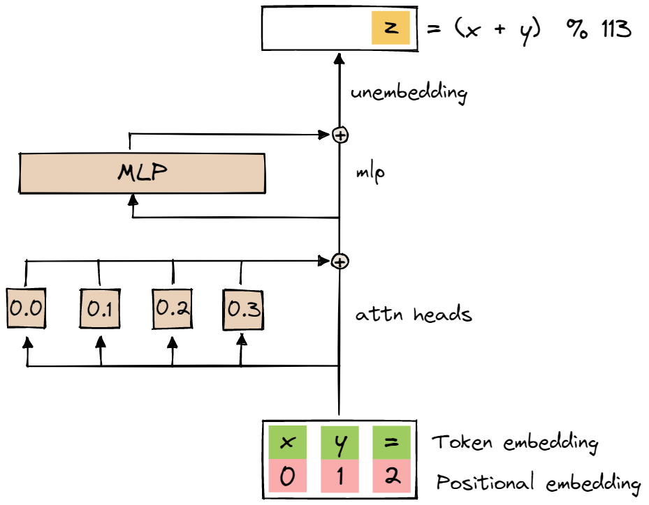
The model we will be reverse-engineering today is a one-layer transformer, with no layer norm and learned positional embeddings. $d_{model} = 128$, $n_{heads} = 4$, $d_{head}=32$, $d_{mlp}=512$.
The task this model was trained on is addition modulo the prime $p = 113$. The input format is a sequence of three tokens [x, y, =], with $d_{vocab}=114$ (integers from $0$ to $p - 1$ and $=$). The prediction for the next token after = should be the token corresponding to $x + y \pmod{p}$.
It was trained with full batch training, with 0.3 of the total data as training data. It is trained with AdamW, with $lr=10^{-3}$ and very high weight decay ($wd=1$).
Summary of the algorithm
Broadly, the algorithm works as follows:
- Given two tokens $x, y \in \{0, 1, \ldots, p - 1\}$, map these to $\sin(\omega x)$, $\cos(\omega x)$, $\sin(\omega y)$, $\cos(\omega y)$, where $\omega = \omega_k = \frac{2k\pi}{p}, k \in \mathbb{N}$.
- In other words, we throw away most frequencies, and only keep a handful of key frequencies corresponding to specific values of $k$.
-
Calcuates the quadratic terms:
$$ \begin{align*} \cos(\omega x) &\cos(\omega y)\\ \sin(\omega x) &\sin(\omega y)\\ \cos(\omega x) &\sin(\omega y)\\ \sin(\omega x) &\cos(\omega y) \end{align*} $$in hacky ways (using attention and ReLU). This also allows us to compute the following linear combinations:$$ \begin{align*} \cos(\omega (x+y)) &= \cos(\omega x) \cos(\omega y) - \sin(\omega x) \sin(\omega y)\\ \sin(\omega (x+y)) &= \sin(\omega x) \cos(\omega y) + \cos(\omega x) \sin(\omega y) \end{align*} $$ -
Computes our output logit vector, s.t. each element $\text{logits}[z]$ is a linear combination of terms of the form:
$$ \cos(\omega (x + y - z)) = \cos(\omega (x+y)) \cos(\omega z) + \sin(\omega (x+y)) \sin(\omega z) $$which is a linear combination of the terms we computed above. - These values (for different $k$) will be added together to get our final output.
- There is constructive interference at $z^* = x + y \; (\operatorname{mod} p)$, and destructive interference everywhere else - hence we get accurate predictions.
Notation
A few words about notation we'll use in these exercises, to help remove ambiguity:
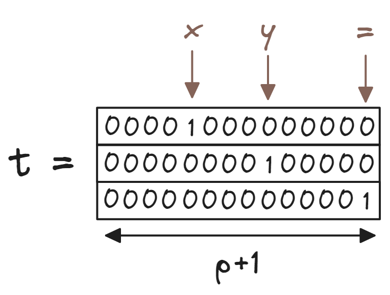
- $x$ and $y$ will always refer to the two inputs to the model. We'll also sometimes use the terminology $t_0$ and $t_1$, which are the one-hot encodings of these inputs.
- The third input token,
=will always be referred to as $t_2$. Unlike $t_0$ and $t_1$, this token is always the same in every input sequence. - $t$ will refer to the matrix of all three one-hot encoded tokens, i.e. it has size $(3, d_{vocab})$. Here, we have $d_{vocab} = p + 1$ (since we have all the numbers from $0$ to $p - 1$, and the token
=.)
- The third input token,
-
$z$ will always refer to the output of the model. For instance, when we talk about the model "computing $\cos(\omega (x + y - z))$", this means that the vector of output logits is the sequence:
$$ (\cos(\omega (x + y - z)))_{z = 0, 1, ..., p-1} $$Note that we discard the logit for the=sign. -
We are keeping TransformerLens' convention of left-multiplying matrices. For instance:
- the embedding matrix $W_E$ has shape $(d_{vocab}, d_{model})$,
- $t_0 ^T W_E \in \mathbb{R}^{d_{model}}$ is the embedding of the first token,
- and $t W_E \in \mathbb{R}^{3 \times d_{model}}$ is the embedding of all three tokens.
Content & Learning Objectives
1️⃣ Periodicity & Fourier basis
This section gets you acquainted with the toy model. You'll do some initial investigations, and see that the activations are highly periodic. You'll also learn how to use the Fourier basis to represent periodic functions.
Learning Objectives
- Understand the problem statement, the model architecture, and the corresponding and functional form of any possible solutions.
- Learn about the Fourier basis (1D and 2D), and how it can be used to represent arbitrary functions.
- Understand that periodic functions are sparse in the Fourier basis, and how this relates to the model's weights.
2️⃣ Circuits & Feature Analysis
In this section, you'll apply your understanding of the Fourier basis and the periodicity of the model's weights to break down the exact algorithm used by the model to solve the task. You'll verify your hypotheses in several different ways.
Learning Objectives
- Apply your understanding of the 1D and 2D Fourier bases to show that the activations / effective weights of your model are highly sparse in the Fourier basis.
- Turn these observations into concrete hypotheses about the model's algorithm.
- Verify these hypotheses using statistical methods, and interventions like ablation.
- Fully understand the model's algorithm, and how it solves the task.
3️⃣ Analysis During Training
In this section, you'll have a look at how the model evolves during the course of training. This section is optional, and the observations we make are more speculative than the rest of the material.
Learning Objectives
- Understand the idea of tracking metrics over time, and how this can inform when certain circuits are forming.
- Investigate and interpret the evolution over time of the singular values of the model's weight matrices.
- Investigate the formation of other capabilities in the model, like commutativity.
☆ Bonus
Finally, we conclude with a discussion of these exercises, and some thoughts on future directions it could be taken.
Setup code
import os
import sys
from functools import partial
from pathlib import Path

import einops
import numpy as np
import torch as t
import torch.nn.functional as F
from huggingface_hub import hf_hub_download
from jaxtyping import Float
from torch import Tensor
from tqdm import tqdm
from transformer_lens import HookedTransformer, HookedTransformerConfig
from transformer_lens.utils import to_numpy

# Make sure exercises are in the path
chapter = "chapter1_transformer_interp"
section = "part52_grokking_and_modular_arithmetic"
root_dir = next(p for p in Path.cwd().parents if (p / chapter).exists())
exercises_dir = root_dir / chapter / "exercises"
section_dir = exercises_dir / section
if str(exercises_dir) not in sys.path:
    sys.path.append(str(exercises_dir))

grokking_root = section_dir / "Grokking"
saved_runs_root = grokking_root / "saved_runs"

import part52_grokking_and_modular_arithmetic.tests as tests
import part52_grokking_and_modular_arithmetic.utils as utils

device = t.device("cuda" if t.cuda.is_available() else "cpu")

t.set_grad_enabled(False)

MAIN = __name__ == "__main__"