3️⃣ Understanding the total elevation circuit

Learning Objectives

• Practice connecting distinctive attention patterns to human-understandable algorithms, and making deductions about model behaviour.
• Understand how MLPs can be viewed as a collection of neurons.
• Build up to a full picture of the total elevation circuit and how it works.

In the largest section of the exercises, you'll examine the attention patterns in different heads, and interpret them as performing some human-understandable algorithm (e.g. copying, or aggregation). You'll use your observations to make deductions about how a particular type of balanced brackets failure mode (mismatched number of left and right brackets) is detected by your model. This is the first time you'll have to deal with MLPs in your models.

This section is quite challenging both from a coding and conceptual perspective, because you need to link the results of your observations and interventions to concrete hypotheses about how the model works.

Attention pattern of the responsible head

Which tokens is 2.0 paying attention to when the query is an open paren at token 0? Recall that we focus on sequences that start with an open paren because sequences that don't can be ruled out immediately, so more sophisticated behavior is unnecessary.

Exercise - get attention probabilities

Write a function that extracts the attention patterns for a given head when run on a batch of inputs.

def get_attn_probs(
    model: HookedTransformer, data: BracketsDataset, layer: int, head: int
) -> Tensor:
    """
    Returns: (N_SAMPLES, max_seq_len, max_seq_len) tensor that sums to 1 over the last dimension.
    """
    raise NotImplementedError()


tests.test_get_attn_probs(get_attn_probs, model, data_mini)

def get_attn_probs(
    model: HookedTransformer, data: BracketsDataset, layer: int, head: int
) -> Tensor:
    """
    Returns: (N_SAMPLES, max_seq_len, max_seq_len) tensor that sums to 1 over the last dimension.
    """
    return get_activation(model, data.toks, utils.get_act_name("pattern", layer))[:, head, :, :]

Once you've passed the tests, you can plot your results:

attn_probs_20 = get_attn_probs(model, data, 2, 0)  # [batch seqQ seqK]
attn_probs_20_open_query0 = attn_probs_20[data.starts_open].mean(0)[0]

bar(
    attn_probs_20_open_query0,
    title="Avg Attention Probabilities for query 0, first token '(', head 2.0",
    width=700,
    template="simple_white",
    labels={"x": "Sequence position", "y": "Attn prob"},
)

You should see an average attention of around 0.5 on position 1, and an average of about 0 for all other tokens. So 2.0 is just moving information from residual stream 1 to residual stream 0. In other words, 2.0 passes residual stream 1 through its W_OV circuit (after LayerNorming, of course), weighted by some amount which we'll pretend is constant. Importantly, this means that the necessary information for classification must already have been stored in sequence position 1 before this head. The plot thickens!

Identifying meaningful direction before this head

If we make the simplification that the vector moved to sequence position 0 by head 2.0 is just layernorm(x[1]) @ W_OV (where x[1] is the vector in the residual stream before head 2.0, at sequence position 1), then we can do the same kind of logit attribution we did before. Rather than decomposing the input to the final layernorm (at sequence position 0) into the sum of ten components and measuring their contribution in the "pre final layernorm unbalanced direction", we can decompose the input to head 2.0 (at sequence position 1) into the sum of the seven components before head 2.0, and measure their contribution in the "pre head 2.0 unbalanced direction".

Here is an annotated diagram to help better explain exactly what we're doing.

Exercise - calculate the pre-head 2.0 unbalanced direction

Below, you'll be asked to calculate this pre_20_dir, which is the unbalanced direction for inputs into head 2.0 at sequence position 1 (based on the fact that vectors at this sequence position are copied to position 0 by head 2.0, and then used in prediction).

First, you'll implement the function get_WOV, to get the OV matrix for a particular layer and head. Recall that this is the product of the W_O and W_V matrices. Then, you'll use this function to write get_pre_20_dir.

def get_WOV(model: HookedTransformer, layer: int, head: int) -> Float[Tensor, "d_model d_model"]:
    """
    Returns the W_OV matrix for a particular layer and head.
    """
    raise NotImplementedError()


def get_pre_20_dir(model, data) -> Float[Tensor, "d_model"]:
    """
    Returns the direction propagated back through the OV matrix of 2.0 and then through the
    layernorm before the layer 2 attention heads.
    """
    raise NotImplementedError()


tests.test_get_pre_20_dir(get_pre_20_dir, model, data_mini)

def get_WOV(model: HookedTransformer, layer: int, head: int) -> Float[Tensor, "d_model d_model"]:
    """
    Returns the W_OV matrix for a particular layer and head.
    """
    return model.W_V[layer, head] @ model.W_O[layer, head]
def get_pre_20_dir(model, data) -> Float[Tensor, "d_model"]:
    """
    Returns the direction propagated back through the OV matrix of 2.0 and then through the
    layernorm before the layer 2 attention heads.
    """
    W_OV = get_WOV(model, 2, 0)
layer2_ln_fit, r2 = get_ln_fit(model, data, layernorm=model.blocks[2].ln1, seq_pos=1)
    layer2_ln_coefs = t.from_numpy(layer2_ln_fit.coef_).to(device)
pre_final_ln_dir = get_pre_final_ln_dir(model, data)
return layer2_ln_coefs.T @ W_OV @ pre_final_ln_dir

Exercise - compute component magnitudes

Now that you've got the pre_20_dir, you can calculate magnitudes for each of the components that came before. You can refer back to the diagram above if you're confused. Remember to subtract the mean for each component for balanced inputs.

# YOUR CODE HERE - define `out_by_component_in_pre_20_unbalanced_dir` (for all components before head 2.0)
pre_layer2_outputs_seqpos1 = out_by_components[:-3, :, 1, :]
out_by_component_in_pre_20_unbalanced_dir = einops.einsum(
    pre_layer2_outputs_seqpos1,
    get_pre_20_dir(model, data),
    "comp batch emb, emb -> comp batch",
)
out_by_component_in_pre_20_unbalanced_dir -= out_by_component_in_pre_20_unbalanced_dir[
    :, data.isbal
].mean(-1, True)

tests.test_out_by_component_in_pre_20_unbalanced_dir(
    out_by_component_in_pre_20_unbalanced_dir, model, data
)

plotly_utils.hists_per_comp(out_by_component_in_pre_20_unbalanced_dir, data, xaxis_range=(-5, 12))

What do you observe?

Some things to notice

One obvious note - the embeddings graph shows an output of zero, in other words no effect on the classification. This is because the input for this path is just the embedding vector in the 0th sequence position - in other words the [START] token's embedding, which is the same for all inputs.

---

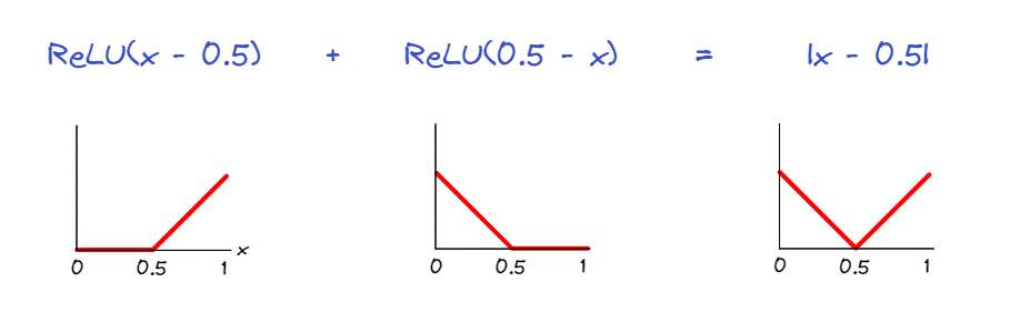
More interestingly, we can see that mlp0 and especially mlp1 are very important. This makes sense -- one thing that mlps are especially capable of doing is turning more continuous features ('what proportion of characters in this input are open parens?') into sharp discontinuous features ('is that proportion exactly 0.5?').

For example, the sum $\operatorname{ReLU}(x-0.5) + \operatorname{ReLU}(0.5-x)$ evaluates to the nonlinear function $|x-0.5|$, which is zero if and only if $x=0.5$. This is one way our model might be able to classify all bracket strings as unbalanced unless they had exactly 50% open parens.

---

Head 1.1 also has some importance, although we will not be able to dig into this today. It turns out that one of the main things it does is incorporate information about when there is a negative elevation failure into this overall elevation branch. This allows the heads to agree the prompt is unbalanced when it is obviously so, even if the overall count of opens and closes would allow it to be balanced.

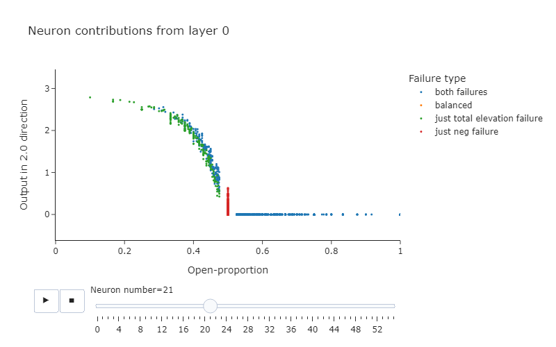
In order to get a better look at what mlp0 and mlp1 are doing more thoughly, we can look at their output as a function of the overall open-proportion.

plotly_utils.mlp_attribution_scatter(
    out_by_component_in_pre_20_unbalanced_dir, data, failure_types_dict
)

MLPs as key-value pairs

When we implemented transformers from scratch, we observed that MLPs can be thought of as key-value pairs. To recap this briefly:

We can write the MLP's output as $f(x^T W^{in})W^{out}$, where $W^{in}$ and $W^{out}$ are the different weights of the MLP (ignoring biases), $f$ is the activation function, and $x$ is a vector in the residual stream. This can be rewritten as:

$$ > f(x^T W^{in}) W^{out} = \sum_{i=1}^{d_{mlp}} f(x^T W^{in}_{[:, i]}) W^{out}_{[i, :]} > $$

We can view the vectors $W^{in}_{[:, i]}$ as the input directions, and $W^{out}_{[i, :]}$ as the output directions. We say the input directions are activated by certain textual features, and when they are activated, vectors are written in the corresponding output direction. This is very similar to the concept of keys and values in attention layers, which is why these vectors are also sometimes called keys and values (e.g. see the paper Transformer Feed-Forward Layers Are Key-Value Memories).

Including biases, the full version of this formula is:

Diagram illustrating this (without biases):

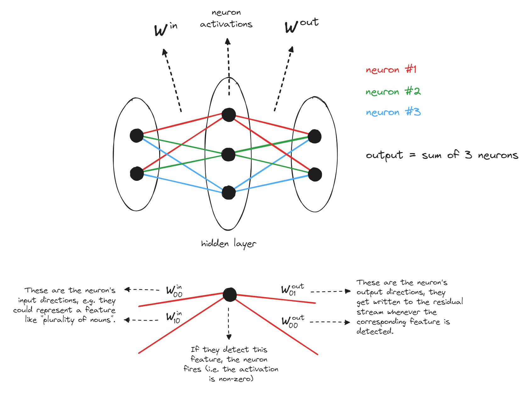
Exercise - get output by neuron

The function get_out_by_neuron should return the given MLP's output per neuron. In other words, the output has shape [batch, seq, neurons, d_model], where out[b, s, i] is the vector $f(\vec x^T W^{in}_{[:,i]} + b^{in}_i)W^{out}_{[i,:]}$ (and summing over i would give you the actual output of the MLP). We ignore $b^{out}$ here, because it isn't attributable to any specific neuron.

When you have this output, you can use get_out_by_neuron_in_20_dir to calculate the output of each neuron in the unbalanced direction for the input to head 2.0 at sequence position 1. Note that we're only considering sequence position 1, because we've observed that head 2.0 is mainly just copying info from position 1 to position 0. This is why we've given you the seq argument in the get_out_by_neuron function, so you don't need to store more information than is necessary.

def get_out_by_neuron(
    model: HookedTransformer, data: BracketsDataset, layer: int, seq: int | None = None
) -> Float[Tensor, "batch *seq neuron d_model"]:
    """
    If seq=None, then out[batch, seq, i, :] = f(x[batch, seq].T @ W_in[:, i] + b_in[i]) @ W_out[i, :],
    i.e. the vector which is written to the residual stream by the ith neuron (where x is the input to
    the residual stream (i.e. shape (batch, seq, d_model)).

    If seq is not None, then out[batch, i, :] = f(x[batch, seq].T @ W_in[:, i]) @ W_out[i, :], i.e. we
    just look at the sequence position given by argument seq.

    (Note, using * in jaxtyping indicates an optional dimension)
    """
    raise NotImplementedError()


def get_out_by_neuron_in_20_dir(
    model: HookedTransformer, data: BracketsDataset, layer: int
) -> Float[Tensor, "batch neurons"]:
    """
    [b, s, i]th element is the contribution of the vector written by the ith neuron to the residual stream in the
    unbalanced direction (for the b-th element in the batch, and the s-th sequence position).

    In other words we need to take the vector produced by the `get_out_by_neuron` function, and project it onto the
    unbalanced direction for head 2.0 (at seq pos = 1).
    """
    raise NotImplementedError()


tests.test_get_out_by_neuron(get_out_by_neuron, model, data_mini)
tests.test_get_out_by_neuron_in_20_dir(get_out_by_neuron_in_20_dir, model, data_mini)

def get_out_by_neuron(
    model: HookedTransformer, data: BracketsDataset, layer: int, seq: int | None = None
) -> Float[Tensor, "batch seq neuron d_model"]:
    """
    If seq=None, then out[batch, seq, i, :] = f(x[batch, seq].T @ W_in[:, i] + b_in[i]) @ W_out[i, :],
    i.e. the vector which is written to the residual stream by the ith neuron (where x is the input to
    the residual stream (i.e. shape (batch, seq, d_model)).
    If seq is not None, then out[batch, i, :] = f(x[batch, seq].T @ W_in[:, i]) @ W_out[i, :], i.e. we
    just look at the sequence position given by argument seq.
    (Note, using  in jaxtyping indicates an optional dimension)
    """
    # Get the W_out matrix for this MLP
    W_out = model.W_out[layer]  # [neuron d_model]
# Get activations of the layer just after the activation function, i.e. this is f(x.T @ W_in)
    f_x_W_in = get_activation(
        model, data.toks, utils.get_act_name("post", layer)
    )  # [batch seq neuron]
# f_x_W_in are activations, so they have batch and seq dimensions - this is where we index by
    # sequence position if not None
    if seq is not None:
        f_x_W_in = f_x_W_in[:, seq, :]  # [batch neuron]
# Calculate the output by neuron (i.e. so summing over the neurons dimension gives the output
    # of the MLP)
    out = einops.einsum(
        f_x_W_in,
        W_out,
        "... neuron, neuron d_model -> ... neuron d_model",
    )
    return out
def get_out_by_neuron_in_20_dir(
    model: HookedTransformer, data: BracketsDataset, layer: int
) -> Float[Tensor, "batch neurons"]:
    """
    [b, s, i]th element is the contribution of the vector written by the ith neuron to the residual stream in the
    unbalanced direction (for the b-th element in the batch, and the s-th sequence position).
    In other words we need to take the vector produced by the get_out_by_neuron function, and project it onto the
    unbalanced direction for head 2.0 (at seq pos = 1).
    """
    # Get neuron output at sequence position 1
    out_by_neuron_seqpos1 = get_out_by_neuron(model, data, layer, seq=1)
# For each neuron, project the vector it writes to residual stream along the pre-2.0 unbalanced
    # direction
    return einops.einsum(
        out_by_neuron_seqpos1,
        get_pre_20_dir(model, data),
        "batch neuron d_model, d_model -> batch neuron",
    )

Exercise - implement the same function, using less memory

This exercise isn't as important as the previous one, and you can skip it if you don't find this interesting (although you're still recommended to look at the solutions, so you understand what's going on here.)

If the only thing we want from the MLPs are their contribution in the unbalanced direction, then we can actually do this without having to store the out_by_neuron_in_20_dir object. Try and find this method, and implement it below.

These kind of ideas aren't vital when working with toy models, but they become more important when working with larger models, and we need to be mindful of memory constraints.

def get_out_by_neuron_in_20_dir_less_memory(
    model: HookedTransformer, data: BracketsDataset, layer: int
) -> Float[Tensor, "batch neurons"]:
    """
    Has the same output as `get_out_by_neuron_in_20_dir`, but uses less memory (because it never
    stores the output vector of each neuron individually).
    """
    raise NotImplementedError()


tests.test_get_out_by_neuron_in_20_dir_less_memory(
    get_out_by_neuron_in_20_dir_less_memory, model, data_mini
)

def get_out_by_neuron_in_20_dir_less_memory(
    model: HookedTransformer, data: BracketsDataset, layer: int
) -> Float[Tensor, "batch neurons"]:
    """
    Has the same output as get_out_by_neuron_in_20_dir, but uses less memory (because it never
    stores the output vector of each neuron individually).
    """
    W_out = model.W_out[layer]  # [neurons d_model]
f_x_W_in = get_activation(model, data.toks, utils.get_act_name("post", layer))[
        :, 1, :
    ]  # [batch neurons]
pre_20_dir = get_pre_20_dir(model, data)  # [d_model]
# Multiply along the d_model dimension
    W_out_in_20_dir = W_out @ pre_20_dir  # [neurons]
    # Multiply elementwise, over neurons (we're broadcasting along the batch dim)
    out_by_neuron_in_20_dir = f_x_W_in * W_out_in_20_dir  # [batch neurons]
return out_by_neuron_in_20_dir

Interpreting the neurons

Now, try to identify several individual neurons that are especially important to 2.0.

For instance, you can do this by seeing which neurons have the largest difference between how much they write in our chosen direction on balanced and unbalanced sequences (especially unbalanced sequences beginning with an open paren).

Use the plot_neurons function to get a sense of what an individual neuron does on differen open-proportions.

One note: now that we are deep in the internals of the network, our assumption that a single direction captures most of the meaningful things going on in this overall-elevation circuit is highly questionable. This is especially true for using our 2.0 direction to analyize the output of mlp0, as one of the main ways this mlp has influence is through more indirect paths (such as mlp0 -> mlp1 -> 2.0) which are not the ones we chose our direction to capture. Thus, it is good to be aware that the intuitions you get about what different layers or neurons are doing are likely to be incomplete.

Note - we've supplied the default argument renderer="browser", which causes the plots to open in a browser rather than in VSCode. This often works better, with less lag (especially in notebooks), but you can remove this if you prefer.

for layer in range(2):
    # Get neuron significances for head 2.0, sequence position #1 output
    neurons_in_unbalanced_dir = get_out_by_neuron_in_20_dir_less_memory(model, data, layer)[
        utils.to_numpy(data.starts_open), :
    ]

    # Plot neurons' activations
    plotly_utils.plot_neurons(neurons_in_unbalanced_dir, model, data, failure_types_dict, layer)

Some observations:

The important neurons in layer 1 can be put into three broad categories:

- Some neurons detect when the open-proportion is greater than 1/2. As a few examples, look at neurons 1.53, 1.39, 1.8 in layer 1. There are some in layer 0 as well, such as 0.33 or 0.43. Overall these seem more common in Layer 1.

- Some neurons detect when the open-proportion is less than 1/2. For instance, neurons 0.21, and 0.7. These are much more rare in layer 1, but you can see some such as 1.50 and 1.6.

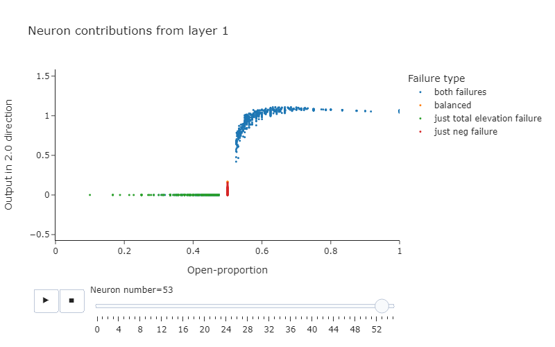
- The network could just use these two types of neurons, and compose them to measure if the open-proportion exactly equals 1/2 by adding them together. But we also see in layer 1 that there are many neurons that output this composed property. As a few examples, look at 1.10 and 1.3. - It's much harder for a single neuron in layer 0 to do this by themselves, given that ReLU is monotonic and it requires the output to be a non-monotonic function of the open-paren proportion. It is possible, however, to take advantage of the layernorm before mlp0 to approximate this -- 0.19 and 0.34 are good examples of this.

Note, there are some neurons which appear to work in the opposite direction (e.g. 0.0). It's unclear exactly what the function of these neurons is (especially since we're only analysing one particular part of one of our model's circuits, so our intuitions about what a particular neuron does might be incomplete). However, what is clear and unambiguous from this plot is that our neurons seem to be detecting the open proportion of brackets, and responding differently if the proportion is strictly more / strictly less than 1/2. And we can see that a large number of these seem to have their main impact via being copied in head 2.0.

---

Below: plots of neurons 0.21 and 1.53. You can observe the patterns described above.

Understanding how the open-proportion is calculated - Head 0.0

Up to this point we've been working backwards from the logits and through the internals of the network. We'll now change tactics somewhat, and start working from the input embeddings forwards. In particular, we want to understand how the network calcuates the open-proportion of the sequence in the first place!

The key will end up being head 0.0. Let's start by examining its attention pattern.

0.0 Attention Pattern

We want to play around with the attention patterns in our heads. For instance, we'd like to ask questions like "what do the attention patterns look like when the queries are always left-parens?". To do this, we'll write a function that takes in a parens string, and returns the q and k vectors (i.e. the values which we take the inner product of to get the attention scores).

Exercise - extracting queries and keys using hooks

def get_q_and_k_for_given_input(
    model: HookedTransformer,
    tokenizer: SimpleTokenizer,
    parens: str,
    layer: int,
) -> tuple[Float[Tensor, "seq n_heads d_model"], Float[Tensor, "seq n_heads d_model"]]:
    """
    Returns the queries and keys for the given parens string, for all attn heads in the given layer.
    """
    raise NotImplementedError()


tests.test_get_q_and_k_for_given_input(get_q_and_k_for_given_input, model, tokenizer)

def get_q_and_k_for_given_input(
    model: HookedTransformer,
    tokenizer: SimpleTokenizer,
    parens: str,
    layer: int,
) -> tuple[Float[Tensor, "seq n_heads d_model"], Float[Tensor, "seq n_heads d_model"]]:
    """
    Returns the queries and keys for the given parens string, for all attn heads in the given layer.
    """
    q_name = utils.get_act_name("q", layer)
    k_name = utils.get_act_name("k", layer)
activations = get_activations(model, tokenizer.tokenize(parens), [q_name, k_name])
return activations[q_name][0], activations[k_name][0]

Activation Patching

Now, we'll introduce the valuable tool of activation patching. This was first introduced in David Bau and Kevin Meng's excellent ROME paper, there called causal tracing.

The setup of activation patching is to take two runs of the model on two different inputs, the clean run and the corrupted run. The clean run outputs the correct answer and the corrupted run does not. The key idea is that we give the model the corrupted input, but then intervene on a specific activation and patch in the corresponding activation from the clean run (i.e. replace the corrupted activation with the clean activation), and then continue the run.

One of the common use-cases for activation patching is to compare the model's performance in clean vs patched runs. If the performance degrades with patching, this is a strong signal that the place you patched in is important for the model's computation. The ability to localise is a key move in mechanistic interpretability - if the computation is diffuse and spread across the entire model, it is likely much harder to form a clean mechanistic story for what's going on. But if we can identify precisely which parts of the model matter, we can then zoom in and determine what they represent and how they connect up with each other, and ultimately reverse engineer the underlying circuit that they represent.

However, here our path patching serves a much simpler purpose - we'll be patching at the query vectors of head 0.0 with values from a sequence of all left-parens, and at the key vectors with the average values from all left and all right parens. This allows us to get a sense for the average attention patterns paid by left-brackets to the rest of the sequence.

We'll write functions to do this for both heads in layer 0, because it will be informative to compare the two.

layer = 0
all_left_parens = "".join(["(" * 40])
all_right_parens = "".join([")" * 40])

model.reset_hooks()
q0_all_left, k0_all_left = get_q_and_k_for_given_input(model, tokenizer, all_left_parens, layer)
q0_all_right, k0_all_right = get_q_and_k_for_given_input(
    model, tokenizer, all_right_parens, layer
)
k0_avg = (k0_all_left + k0_all_right) / 2

# Define hook function to patch in q or k vectors
def hook_fn_patch_qk(
    value: Float[Tensor, "batch seq head d_head"],
    hook: HookPoint,
    new_value: Float[Tensor, "... seq d_head"],
    head_idx: int | None = None,
) -> None:
    if head_idx is not None:
        value[..., head_idx, :] = new_value[..., head_idx, :]
    else:
        value[...] = new_value[...]


# Define hook function to display attention patterns (using plotly)
def hook_fn_display_attn_patterns(
    pattern: Float[Tensor, "batch heads seqQ seqK"], hook: HookPoint, head_idx: int = 0
) -> None:
    avg_head_attn_pattern = pattern.mean(0)
    labels = ["[start]", *[f"{i + 1}" for i in range(40)], "[end]"]
    display(
        cv.attention.attention_heads(
            tokens=labels,
            attention=avg_head_attn_pattern,
            attention_head_names=["0.0", "0.1"],
            max_value=avg_head_attn_pattern.max(),
            mask_upper_tri=False,  # use for bidirectional models
        )
    )


# Run our model on left parens, but patch in the average key values for left vs right parens
# This is to give us a rough idea how the model behaves on average when the query is a left paren
model.run_with_hooks(
    tokenizer.tokenize(all_left_parens).to(device),
    return_type=None,
    fwd_hooks=[
        (utils.get_act_name("k", layer), partial(hook_fn_patch_qk, new_value=k0_avg)),
        (utils.get_act_name("pattern", layer), hook_fn_display_attn_patterns),
    ],
)

We are most interested in the attention pattern at query position 1, because this is the position we move information to that is eventually fed into attention head 2.0, then moved to position 0 and used for prediction.

(Note - we've chosen to focus on the scenario when the first paren is an open paren, because the model actually deals with bracket strings that open with a right paren slightly differently - these are obviously unbalanced, so a complicated mechanism is unnecessary.)

Let's plot a bar chart of the attention probability paid by the the open-paren query at position 1 to all the other positions. Here, rather than patching in both the key and query from artificial sequences, we're running the model on our entire dataset and patching in an artificial value for just the query (all open parens). Both methods are reasonable here, since we're just looking for a general sense of how our query vector at position 1 behaves when it's an open paren.

def hook_fn_display_attn_patterns_for_single_query(
    pattern: Float[Tensor, "batch heads seqQ seqK"],
    hook: HookPoint,
    head_idx: int = 0,
    query_idx: int = 1,
):
    bar(
        utils.to_numpy(pattern[:, head_idx, query_idx].mean(0)),
        title="Average attn probabilities on data at posn 1, with query token = '('",
        labels={"index": "Sequence position of key", "value": "Average attn over dataset"},
        height=500,
        width=800,
        yaxis_range=[0, 0.1],
        template="simple_white",
    )


data_len_40 = BracketsDataset.with_length(data_tuples, 40).to(device)

model.reset_hooks()
model.run_with_hooks(
    data_len_40.toks[data_len_40.isbal],
    return_type=None,
    fwd_hooks=[
        (utils.get_act_name("q", 0), partial(hook_fn_patch_qk, new_value=q0_all_left)),
        (utils.get_act_name("pattern", 0), hook_fn_display_attn_patterns_for_single_query),
    ],
)

Proposing a hypothesis

Before we connect all the pieces together, let's list the facts that we know about our model so far (going chronologically from our observations):

• Attention head 2.0 seems to be largely responsible for classifying brackets as unbalanced when they have non-zero net elevation (i.e. have a different number of left and right parens).
  • Attention head 2.0 attends strongly to the sequence position $i=1$, in other words it's pretty much just moving the residual stream vector from position 1 to position 0 (and applying matrix $W_{OV}$).
  • So there must be earlier components of the model which write to sequence position 1, in a way which influences the model to make correct classifications (via the path through head 2.0).
• There are several neurons in MLP0 and MLP1 which seem to calculate a nonlinear function of the open parens proportion - some of them are strongly activating when the proportion is strictly greater than $1/2$, others when it is strictly smaller than $1/2$.
• If the query token in attention head 0.0 is an open paren, then it attends to all key positions after $i$ with roughly equal magnitude.
  • In particular, this holds for the sequence position $i=1$, which attends approximately uniformly to all sequence positions.

Based on all this, can you formulate a hypothesis for how the elevation circuit works, which ties all three of these observations together?

At this point, we've pretty much empirically verified all the observations above. One thing we haven't really proven yet is that (1) is working as we've described above. We want to verify that head 0.0 is calculating some kind of difference between the number of left and right brackets, and writing this information to the residual stream. In the next section, we'll find a way to test this hypothesis.

The 0.0 OV circuit

We want to understand what the 0.0 head is writing to the residual stream. In particular, we are looking for evidence that it is writing information about the net elevation.

We've already seen that query position 1 is attending approximately uniformly to all key positions. This means that (ignoring start and end tokens) the vector written to position 1 is approximately:

where $L$ is the linear approximation for the layernorm before the first attention layer, and $x$ is the (seq_len, d_model)-size residual stream consisting of vectors ${\color{orange}{x_i}}$ for each sequence position $i$.

We can write ${\color{orange}{x_j}} = {\color{orange}{pos_j}} + {\color{orange}{tok_j}}$, where ${\color{orange}{pos_j}}$ and ${\color{orange}{tok_j}}$ stand for the positional and token embeddings respectively. So this gives us:

where $n_L$ and $n_R$ are the number of left and right brackets respectively, and ${\color{orange}{\vec v_L}}, {\color{orange}{\vec v_R}}$ are the images of the token embeddings for left and right parens respectively under the image of the layernorm and OV circuit:

where ${\color{orange}{LeftParen}}$ and ${\color{orange}{RightParen}}$ are the token embeddings for left and right parens respectively.

Finally, we have an ability to formulate a test for our hypothesis in terms of the expression above:

If head 0.0 is performing some kind of aggregation, then we should see that ${\color{orange}\vec v_L}$ and ${\color{orange}\vec v_R}$ are vectors pointing in opposite directions. In other words, head 0.0 writes some scalar multiple of vector $v$ to the residual stream, and we can extract the information $n_L - n_R$ by projecting in the direction of this vector. The MLP can then take this information and process it in a nonlinear way, writing information about whether the sequence is balanced to the residual stream.

Exercise - validate the hypothesis

Here, you should show that the two vectors have cosine similarity close to -1, demonstrating that this head is "tallying" the open and close parens that come after it.

You can fill in the function embedding (to return the token embedding vector corresponding to a particular character, i.e. the vectors we've called ${\color{orange}LeftParen}$ and ${\color{orange}RightParen}$ above), which will help when computing these vectors.

def embedding(
    model: HookedTransformer, tokenizer: SimpleTokenizer, char: str
) -> Float[Tensor, "d_model"]:
    assert char in ("(", ")")
    idx = tokenizer.t_to_i[char]
    return model.W_E[idx]


# YOUR CODE HERE - define v_L and v_R, as described above.

print(f"Cosine similarity: {t.cosine_similarity(v_L, v_R, dim=0).item():.4f}")

Cosine similarity:  -0.9974

W_OV = model.W_V[0, 0] @ model.W_O[0, 0]
layer0_ln_fit = get_ln_fit(model, data, layernorm=model.blocks[0].ln1, seq_pos=None)[0]
layer0_ln_coefs = t.from_numpy(layer0_ln_fit.coef_).to(device)
v_L = embedding(model, tokenizer, "(") @ layer0_ln_coefs.T @ W_OV
v_R = embedding(model, tokenizer, ")") @ layer0_ln_coefs.T @ W_OV
print(f"Cosine similarity: {t.cosine_similarity(v_L, v_R, dim=0).item():.4f}")

Exercise - cosine similarity of input directions (optional)

Another way we can get evidence for this hypothesis - recall in our discussion of MLP neurons that $W^{in}_{[:,i]}$ (the $i$th column of matrix $W^{in}$, where $W^{in}$ is the first linear layer of the MLP) is a vector representing the "in-direction" of the neuron. If these neurons are indeed measuring open/closed proportions in the way we think, then we should expect to see the vectors $v_R$, $v_L$ have high dot product with these vectors.

Investigate this by filling in the two functions below. cos_sim_with_MLP_weights returns the vector of cosine similarities between a vector and the columns of $W^{in}$ for a given layer, and avg_squared_cos_sim returns the average squared cosine similarity between a vector $v$ and a randomly chosen vector with the same size as $v$ (we can choose this vector in any sensible way, e.g. sampling it from the iid normal distribution then normalizing it). You should find that the average squared cosine similarity per neuron between $v_R$ and the in-directions for neurons in MLP0 and MLP1 is much higher than you would expect by chance.

def cos_sim_with_MLP_weights(
    model: HookedTransformer, v: Float[Tensor, "d_model"], layer: int
) -> Float[Tensor, "d_mlp"]:
    """
    Returns a vector of length d_mlp, where the ith element is the cosine similarity between v and
    the ith in-direction of the MLP in layer `layer`.

    Recall that the in-direction of the MLPs are the columns of the W_in matrix.
    """
    raise NotImplementedError()


def avg_squared_cos_sim(v: Float[Tensor, "d_model"], n_samples: int = 1000) -> float:
    """
    Returns the average (over n_samples) cosine similarity between v and another randomly chosen
    vector of length `d_model`.

    We can create random vectors from the standard N(0, I) distribution.
    """
    raise NotImplementedError()


print("Avg squared cosine similarity of v_R with ...\n")

cos_sim_mlp0 = cos_sim_with_MLP_weights(model, v_R, 0)
print(f"...MLP input directions in layer 0: {cos_sim_mlp0.pow(2).mean():.4f}")

cos_sim_mlp1 = cos_sim_with_MLP_weights(model, v_R, 1)
print(f"...MLP input directions in layer 1: {cos_sim_mlp1.pow(2).mean():.4f}")

cos_sim_rand = avg_squared_cos_sim(v_R)
print(f"...random vectors of len = d_model: {cos_sim_rand:.4f}")

Avg squared cosine similarity of v_R with ...
...MLP input directions in layer 0: 0.1239
...MLP input directions in layer 1: 0.1301
...random vectors of len = d_model: 0.0179

def cos_sim_with_MLP_weights(
    model: HookedTransformer, v: Float[Tensor, "d_model"], layer: int
) -> Float[Tensor, "d_mlp"]:
    """
    Returns a vector of length d_mlp, where the ith element is the cosine similarity between v and
    the ith in-direction of the MLP in layer layer.
    Recall that the in-direction of the MLPs are the columns of the W_in matrix.
    """
    v_unit = v / v.norm()
    W_in_unit = model.W_in[layer] / model.W_in[layer].norm(dim=0)
return einops.einsum(v_unit, W_in_unit, "d_model, d_model d_mlp -> d_mlp")
def avg_squared_cos_sim(v: Float[Tensor, "d_model"], n_samples: int = 1000) -> float:
    """
    Returns the average (over n_samples) cosine similarity between v and another randomly chosen
    vector of length d_model.
    We can create random vectors from the standard N(0, I) distribution.
    """
    v2 = t.randn(n_samples, v.shape[0]).to(device)
    v2 /= v2.norm(dim=1, keepdim=True)
v1 = v / v.norm()
return (v1 * v2).pow(2).sum(1).mean().item()

As an extra-bonus exercise, you can also compare the squared cosine similarities per neuron to your neuron contribution plots you made earlier (the ones with sliders). Do the neurons which have particularly high cosine similarity with $v_R$ correspond to the neurons which write to the unbalanced direction of head 2.0 in a big way whenever the proportion of open parens is not 0.5? (This would provide further evidence that the main source of information about total open proportion of brackets which is used in the net elevation circuit is provided by the multiples of $v_R$ and $v_L$ written to the residual stream by head 0.0). You can go back to your old plots and check.

Summary

Great! Let's stop and take stock of what we've learned about this circuit.

Head 0.0 pays attention uniformly to the suffix following each token, tallying up the amount of open and close parens that it sees and writing that value to the residual stream. This means that it writes a vector representing the total elevation to residual stream 1. The MLPs in residual stream 1 then operate nonlinearly on this tally, writing vectors to the residual stream that distinguish between the cases of zero and non-zero total elevation. Head 2.0 copies this signal to residual stream 0, where it then goes through the classifier and leads to a classification as unbalanced. Our first-pass understanding of this behavior is complete.

An illustration of this circuit is given below. It's pretty complicated with a lot of moving parts, so don't worry if you don't follow all of it!

Key: the thick black lines and orange dotted lines show the paths through our transformer constituting the elevation circuit. The orange dotted lines indicate the skip connections. Each of the important heads and MLP layers are coloured bold. The three important parts of our circuit (head 0.0, the MLP layers, and head 2.0) are all give annotations explaining what they're doing, and the evidence we found for this.