2️⃣ Moving backwards

Learning Objectives

• Understand how to perform logit attribution.
• Understand how to work backwards through a model to identify which components matter most for the final classification probabilities.
• Understand how LayerNorm works, and look at some ways to deal with it in your models.

Here, you'll perform logit attribution, and learn how to work backwards through particular paths of a model to figure out which components matter most for the final classification probabilities. This is the first time you'll have to deal with LayerNorm in your models.

This section should be familiar if you've done logit attribution for induction heads (although these exercises are slightly more challenging from a coding perspective). The LayerNorm-based exercises are a bit fiddly!

Suppose we run the model on some sequence and it outputs the classification probabilities [0.99, 0.01], i.e. highly confident classification as "unbalanced".

We'd like to know why the model had this output, and we'll do so by moving backwards through the network, and figuring out the correspondence between facts about earlier activations and facts about the final output. We want to build a chain of connections through different places in the computational graph of the model, repeatedly reducing our questions about later values to questions about earlier values.

Let's start with an easy one. Notice that the final classification probabilities only depend on the difference between the class logits, as softmax is invariant to constant additions. So rather than asking, "What led to this probability on balanced?", we can equivalently ask, "What led to this difference in logits?". Let's move another step backward. Since the logits are each a linear function of the output of the final LayerNorm, their difference will be some linear function as well. In other words, we can find a vector in the space of LayerNorm outputs such that the logit difference will be the dot product of the LayerNorm's output with that vector.

We now want some way to tell which parts of the model are doing something meaningful. We will do this by identifying a single direction in the embedding space of the start token that we claim to be the "unbalanced direction": the direction that most indicates that the input string is unbalanced. It is important to note that it might be that other directions are important as well (in particular because of layer norm), but for a first approximation this works well.

We'll do this by starting from the model outputs and working backwards, finding the unbalanced direction at each stage.

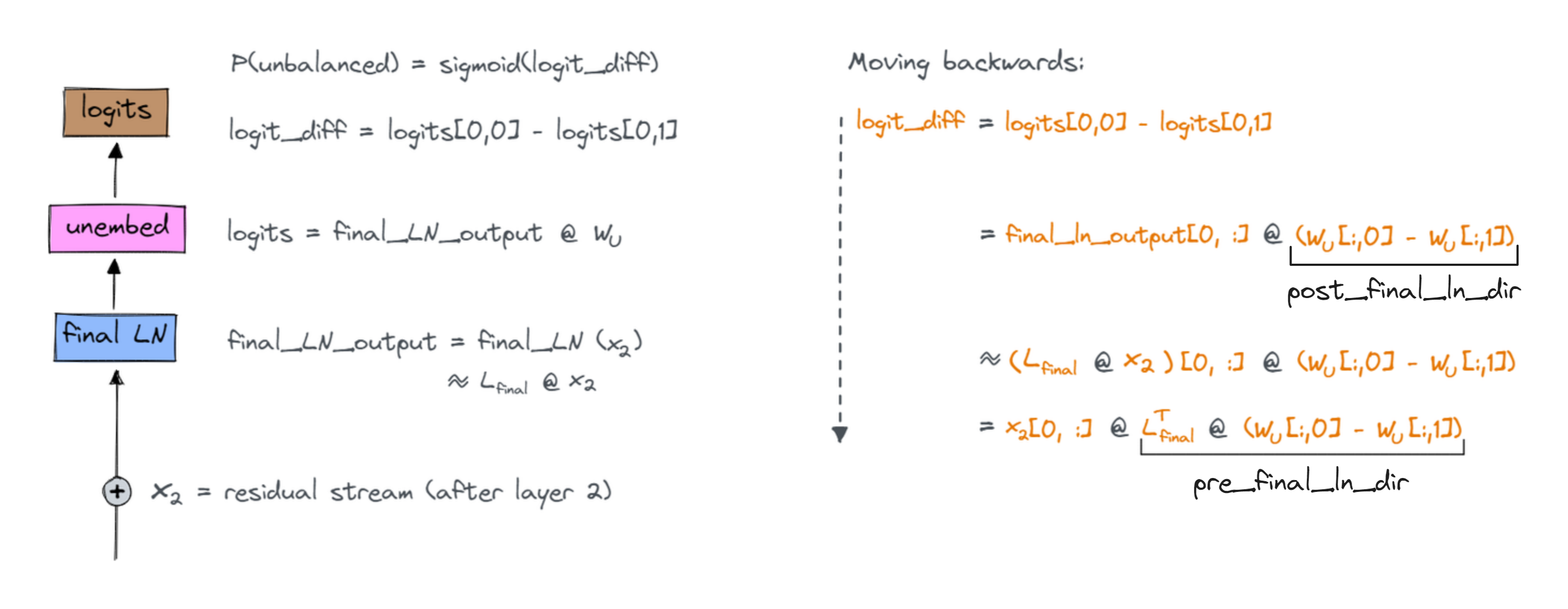
Moving back to the residual stream

The final part of the model is the classification head, which has three stages - the final layernorm, the unembedding, and softmax, at the end of which we get our probabilities.

Note - for simplicity, we'll ignore the batch dimension in the following discussion.

Some notes on the shapes of the objects in the diagram:

• x_2 is the vector in the residual stream after layer 2's attention heads and MLPs. It has shape (seq_len, d_model).
• final_ln_output has shape (seq_len, d_model).
• W_U has shape (d_model, 2), and so logits has shape (seq_len, 2).
• We get P(unbalanced) by taking the 0th element of the softmaxed logits, for sequence position 0.

Stage 1: Translating through softmax

Let's get P(unbalanced) as a function of the logits. Luckily, this is easy. Since we're doing the softmax over two elements, it simplifies to the sigmoid of the difference of the two logits:

Since sigmoid is monotonic, a large value of $\hat{y}_0$ follows from logits with a large $\text{logit}_0 - \text{logit}_1$. From now on, we'll only ask "What leads to a large difference in logits?"

Stage 2: Translating through linear

The next step we encounter is the decoder: logits = final_LN_output @ W_U, where

• W_U has shape (d_model, 2)
• final_LN_output has shape (seq_len, d_model)

We can now put the difference in logits as a function of $W$ and $x_{\text{linear}}$ like this:

logit_diff = (final_LN_output @ W_U)[0, 0] - (final_LN_output @ W_U)[0, 1]
           = final_LN_output[0, :] @ (W_U[:, 0] - W_U[:, 1])

(recall that the (i, j)th element of matrix AB is A[i, :] @ B[:, j])

So a high difference in the logits follows from a high dot product of the output of the LayerNorm with the corresponding unembedding vector. We'll call this the post_final_ln_dir, i.e. the unbalanced direction for values in the residual stream after the final layernorm.

Exercise - get the post_final_ln_dir

In the function below, you should compute this vector (this should just be a one-line function).

def get_post_final_ln_dir(model: HookedTransformer) -> Float[Tensor, "d_model"]:
    """
    Returns the direction in which final_ln_output[0, :] should point to maximize P(unbalanced)
    """
    raise NotImplementedError()


tests.test_get_post_final_ln_dir(get_post_final_ln_dir, model)

def get_post_final_ln_dir(model: HookedTransformer) -> Float[Tensor, "d_model"]:
    """
    Returns the direction in which final_ln_output[0, :] should point to maximize P(unbalanced)
    """
    return model.W_U[:, 0] - model.W_U[:, 1]

Stage 3: Translating through LayerNorm

We want to find the unbalanced direction before the final layer norm, since this is where we can write the residual stream as a sum of terms. LayerNorm messes with this sort of direction analysis, since it is nonlinear. For today, however, we will approximate it with a linear fit. This is good enough to allow for interesting analysis (see for yourself that the $R^2$ values are very high for the fit)!

With a linear approximation to LayerNorm, which I'll use the matrix L_final for, we can translate "What is the dot product of the output of the LayerNorm with the unbalanced-vector?" to a question about the input to the LN. We simply write:

final_ln_output[0, :] = final_ln(x_linear[0, :])
                      = L_final @ x_linear[0, :]

Summary

We can use the logit diff as a measure of how strongly our model is classifying a bracket string as unbalanced (higher logit diff = more certain that the string is unbalanced).

We can approximate logit diff as a linear function of pre_final_ln_dir (because the unembedding is linear, and the layernorm is approximately linear). This means we can approximate logit diff as the dot product of post_final_ln_dir with the residual stream value before the final layernorm. If we could find this post_final_ln_dir, then we could start to answer other questions like which components' output had the highest dot product with this value.

The diagram below shows how we can step back through the model to find our unbalanced direction pre_final_ln_dir. Notation: $x_2$ refers to the residual stream value after layer 2's attention heads and MLPs (i.e. just before the last layernorm), and $L_{final}$ is the linear approximation of the final layernorm.

Exercise - get the pre_final_ln_dir

Ideally, we would calculate pre_final_ln_dir directly from the model's weights, like we did for post_final_ln_dir. Unfortunately, it's not so easy in this case, because in order to get our linear approximation L_final, we need to fit a linear regression with actual data that gets passed through the model.

Below, you should implement the function get_ln_fit to fit a linear regression to the inputs and outputs of one of your model's layernorms, and then get_pre_final_ln_dir which estimates the value of pre_final_ln_dir (as annotated in the diagram above).

We've given you a few helper functions:

• get_activation(s), which use the run_with_cache function to return one or several activations for a given batch of tokens
• LN_hook_names, which takes a layernorm in the model (e.g. model.ln_final) and returns the names of the hooks immediately before or after the layernorm. This will be useful in the get_activation(s) function, when you want to refer to these values (since your linear regression will be fitted on the inputs and outputs to your model's layernorms).

When it comes to fitting the regression, we recommend using the sklearn LinearRegression class to find a linear fit to the inputs and outputs of your model's layernorms. You should include a fit coefficient in your regression (this is the default for LinearRegression).

Note, we have the seq_pos argument because sometimes we'll want to fit the regression over all sequence positions and sometimes we'll only care about some and not others (e.g. for the final layernorm in the model, we only care about the 0th position because that's where we take the prediction from; all other positions are discarded).

def get_activations(
    model: HookedTransformer, toks: Int[Tensor, "batch seq"], names: list[str]
) -> ActivationCache:
    """Uses hooks to return activations from the model, in the form of an ActivationCache."""
    names_list = [names] if isinstance(names, str) else names
    _, cache = model.run_with_cache(
        toks,
        return_type=None,
        names_filter=lambda name: name in names_list,
    )
    return cache


def get_activation(model: HookedTransformer, toks: Int[Tensor, "batch seq"], name: str):
    """Gets a single activation."""
    return get_activations(model, toks, [name])[name]


def LN_hook_names(layernorm: nn.Module) -> tuple[str, str]:
    """
    Returns the names of the hooks immediately before and after a given layernorm.

    Example:
        model.final_ln -> ("blocks.2.hook_resid_post", "ln_final.hook_normalized")
    """
    if layernorm.name == "ln_final":
        input_hook_name = utils.get_act_name("resid_post", 2)
        output_hook_name = "ln_final.hook_normalized"
    else:
        layer, ln = layernorm.name.split(".")[1:]
        input_hook_name = utils.get_act_name("resid_pre" if ln == "ln1" else "resid_mid", layer)
        output_hook_name = utils.get_act_name("normalized", layer, ln)

    return input_hook_name, output_hook_name


def get_ln_fit(
    model: HookedTransformer,
    data: BracketsDataset,
    layernorm: nn.Module,
    seq_pos: int | None = None,
) -> tuple[LinearRegression, float]:
    """
    Fits a linear regression, where the inputs are the values just before the layernorm given by the
    input argument `layernorm`, and the values to predict are the layernorm's outputs.

    if `seq_pos` is None, find best fit aggregated over all sequence positions. Otherwise, fit only
    for the activations at `seq_pos`.

    Returns: A tuple of a (fitted) sklearn LinearRegression object and the r^2 of the fit.
    """
    raise NotImplementedError()


tests.test_get_ln_fit(get_ln_fit, model, data_mini)

_, r2 = get_ln_fit(model, data, layernorm=model.ln_final, seq_pos=0)
print(f"r^2 for LN_final, at sequence position 0: {r2:.4f}")
_, r2 = get_ln_fit(model, data, layernorm=model.blocks[1].ln1, seq_pos=None)
print(f"r^2 for LN1, layer 1, over all sequence positions: {r2:.4f}")

def get_ln_fit(
    model: HookedTransformer,
    data: BracketsDataset,
    layernorm: nn.Module,
    seq_pos: int | None = None,
) -> tuple[LinearRegression, float]:
    """
    Fits a linear regression, where the inputs are the values just before the layernorm given by the
    input argument layernorm, and the values to predict are the layernorm's outputs.
    if seq_pos is None, find best fit aggregated over all sequence positions. Otherwise, fit only
    for the activations at seq_pos.
    Returns: A tuple of a (fitted) sklearn LinearRegression object and the r^2 of the fit.
    """
    input_hook_name, output_hook_name = LN_hook_names(layernorm)
activations_dict = get_activations(model, data.toks, [input_hook_name, output_hook_name])
    inputs = utils.to_numpy(activations_dict[input_hook_name])
    outputs = utils.to_numpy(activations_dict[output_hook_name])
if seq_pos is None:
        inputs = einops.rearrange(inputs, "batch seq d_model -> (batch seq) d_model")
        outputs = einops.rearrange(outputs, "batch seq d_model -> (batch seq) d_model")
    else:
        inputs = inputs[:, seq_pos, :]
        outputs = outputs[:, seq_pos, :]
final_ln_fit = LinearRegression().fit(inputs, outputs)
r2 = final_ln_fit.score(inputs, outputs)
return (final_ln_fit, r2)

3. Calculating pre_final_ln_dir

Armed with our linear fit, we can now identify the direction in the residual stream before the final layer norm that most points in the direction of unbalanced evidence.

def get_pre_final_ln_dir(
    model: HookedTransformer, data: BracketsDataset
) -> Float[Tensor, "d_model"]:
    """
    Returns the direction in residual stream (pre ln_final, at sequence position 0) which
    most points in the direction of making an unbalanced classification.
    """
    raise NotImplementedError()


tests.test_get_pre_final_ln_dir(get_pre_final_ln_dir, model, data_mini)

def get_pre_final_ln_dir(
    model: HookedTransformer, data: BracketsDataset
) -> Float[Tensor, "d_model"]:
    """
    Returns the direction in residual stream (pre ln_final, at sequence position 0) which
    most points in the direction of making an unbalanced classification.
    """
    post_final_ln_dir = get_post_final_ln_dir(model)
final_ln_fit = get_ln_fit(model, data, layernorm=model.ln_final, seq_pos=0)[0]
    final_ln_coefs = t.from_numpy(final_ln_fit.coef_).to(device)
return final_ln_coefs.T @ post_final_ln_dir

Writing the residual stream as a sum of terms

As we've seen in previous exercises, it's much more natural to think about the residual stream as a sum of terms, each one representing a different path through the model. Here, we have ten components which write to the residual stream: the direct path (i.e. the embeddings), and two attention heads and one MLP on each of the three layers. We can write the residual stream as a sum of these terms.

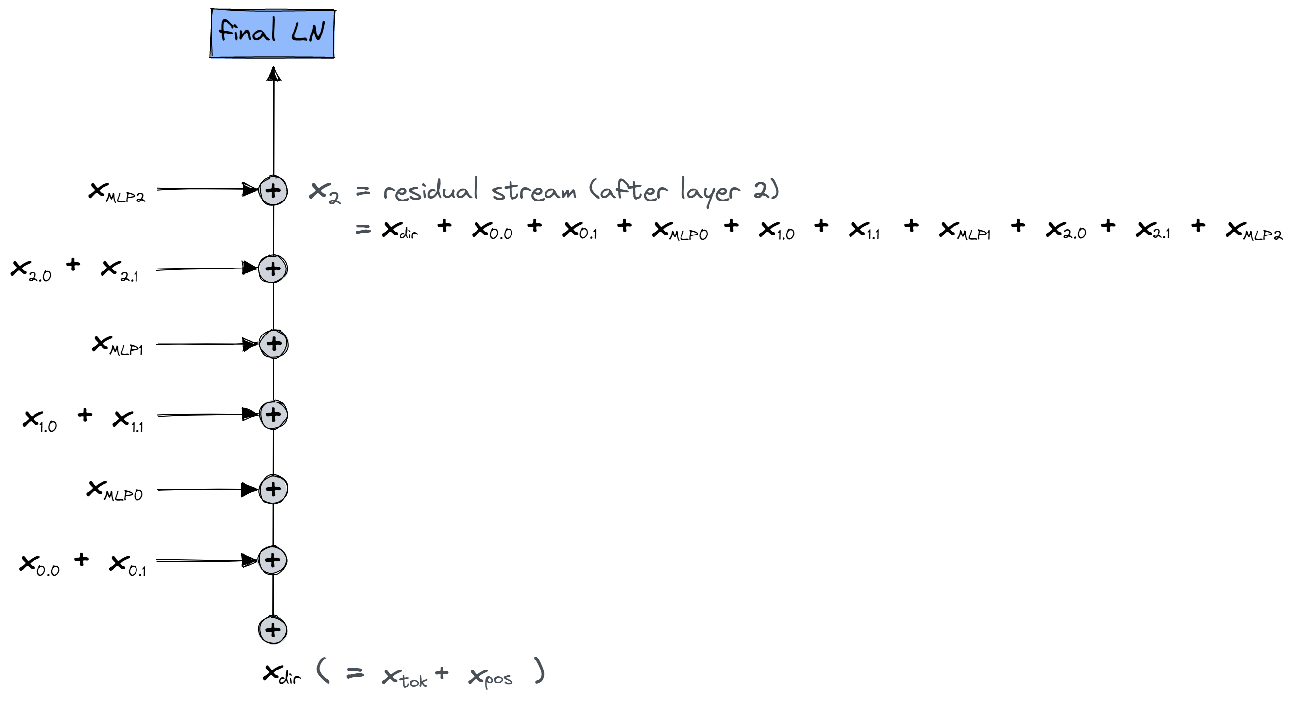
Once we do this, we can narrow in on the components who are making direct contributions to the classification, i.e. which are writing vectors to the residual stream which have a high dot produce with the pre_final_ln_dir for unbalanced brackets relative to balanced brackets.

In order to answer this question, we need the following tools: - A way to break down the input to the LN by component. - A tool to identify a direction in the embedding space that causes the network to output 'unbalanced' (we already have this)

Exercise - breaking down the residual stream by component

Use your get_activations function to create a tensor of shape [num_components, dataset_size, seq_pos], where the number of components = 10.

This is a termwise representation of the input to the final layer norm from each component (recall that we can see each head as writing something to the residual stream, which is eventually fed into the final layer norm). The order of the components in your function's output should be the same as shown in the diagram above (i.e. in chronological order of how they're added to the residual stream).

(The only term missing from the sum of these is the W_O-bias from each of the attention layers).

def get_out_by_components(
    model: HookedTransformer, data: BracketsDataset
) -> Float[Tensor, "component batch seq_pos emb"]:
    """
    Computes a tensor of shape [10, dataset_size, seq_pos, emb] representing the output of the
    model's components when run on the data.

    The first dimension is the stacked components, in the following order:
        [embeddings, head 0.0, head 0.1, mlp 0, head 1.0, head 1.1, mlp 1, head 2.0, head 2.1, mlp 2]
    """
    raise NotImplementedError()


tests.test_get_out_by_components(get_out_by_components, model, data_mini)

def get_out_by_components(
    model: HookedTransformer, data: BracketsDataset
) -> Float[Tensor, "component batch seq_pos emb"]:
    """
    Computes a tensor of shape [10, dataset_size, seq_pos, emb] representing the output of the
    model's components when run on the data.
    The first dimension is the stacked components, in the following order:
        [embeddings, head 0.0, head 0.1, mlp 0, head 1.0, head 1.1, mlp 1, head 2.0, head 2.1, mlp 2]
    """
    embedding_hook_names = ["hook_embed", "hook_pos_embed"]
    head_hook_names = [utils.get_act_name("result", layer) for layer in range(model.cfg.n_layers)]
    mlp_hook_names = [utils.get_act_name("mlp_out", layer) for layer in range(model.cfg.n_layers)]
all_hook_names = embedding_hook_names + head_hook_names + mlp_hook_names
    activations = get_activations(model, data.toks, all_hook_names)
out = (activations["hook_embed"] + activations["hook_pos_embed"]).unsqueeze(0)
for head_hook_name, mlp_hook_name in zip(head_hook_names, mlp_hook_names):
        out = t.concat(
            [
                out,
                einops.rearrange(
                    activations[head_hook_name], "batch seq heads emb -> heads batch seq emb"
                ),
                activations[mlp_hook_name].unsqueeze(0),
            ]
        )
return out

Now, you can test your function by confirming that input to the final layer norm is the sum of the output of each component and the output projection biases.

biases = model.b_O.sum(0)
out_by_components = get_out_by_components(model, data)
summed_terms = out_by_components.sum(dim=0) + biases

final_ln_input_name, final_ln_output_name = LN_hook_names(model.ln_final)
final_ln_input = get_activation(model, data.toks, final_ln_input_name)

t.testing.assert_close(summed_terms, final_ln_input)
print("Tests passed!")

Which components matter?

To figure out which components are directly important for the the model's output being "unbalanced", we can see which components tend to output a vector to the position-0 residual stream with higher dot product in the unbalanced direction for actually unbalanced inputs.

The idea is that, if a component is important for correctly classifying unbalanced inputs, then its vector output when fed unbalanced bracket strings will have a higher dot product in the unbalanced direction than when it is fed balanced bracket strings.

In this section, we'll plot histograms of the dot product for each component. This will allow us to observe which components are significant.

For example, suppose that one of our components produced bimodal output like this:

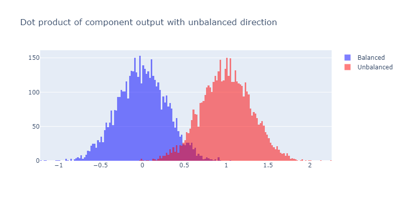
This would be strong evidence that this component is important for the model's output being unbalanced, since it's pushing the unbalanced bracket inputs further in the unbalanced direction (i.e. the direction which ends up contributing to the inputs being classified as unbalanced) relative to the balanced inputs.

Exercise - compute output in unbalanced direction for each component

In the code block below, you should compute a (10, batch)-size tensor called out_by_component_in_unbalanced_dir. The [i, j]th element of this tensor should be the dot product of the ith component's output with the unbalanced direction, for the jth sequence in your dataset.

You should normalize it by subtracting the mean of the dot product of this component's output with the unbalanced direction on balanced samples - this will make sure the histogram corresponding to the balanced samples is centered at 0 (like in the figure above), which will make it easier to interpret. Remember, it's only the difference between the dot product on unbalanced and balanced samples that we care about (since adding a constant to both logits doesn't change the model's probabilistic output).

We've given you a hists_per_comp function which will plot these histograms for you - all you need to do is calculate the out_by_component_in_unbalanced_dir object and supply it to that function.

# YOUR CODE HERE - define the object `out_by_component_in_unbalanced_dir`

tests.test_out_by_component_in_unbalanced_dir(out_by_component_in_unbalanced_dir, model, data)

plotly_utils.hists_per_comp(out_by_component_in_unbalanced_dir, data, xaxis_range=[-10, 20])

# Get output by components, at sequence position 0 (which is used for classification)
out_by_components_seq0 = out_by_components[:, :, 0, :]  # [component=10 batch d_model]
# Get the unbalanced direction for tensors being fed into the final layernorm
pre_final_ln_dir = get_pre_final_ln_dir(model, data)  # [d_model]
# Get the size of the contributions for each component
out_by_component_in_unbalanced_dir = einops.einsum(
    out_by_components_seq0,
    pre_final_ln_dir,
    "comp batch d_model, d_model -> comp batch",
)
# Subtract the mean
out_by_component_in_unbalanced_dir -= (
    out_by_component_in_unbalanced_dir[:, data.isbal].mean(dim=1).unsqueeze(1)
)

Which heads do you think are the most important, and can you guess why that might be?

Head influence by type of failures

Those histograms showed us which heads were important, but it doesn't tell us what these heads are doing, however. In order to get some indication of that, let's focus in on the two heads in layer 2 and see how much they write in our chosen direction on different types of inputs. In particular, we can classify inputs by if they pass the 'overall elevation' and 'nowhere negative' tests.

We'll also ignore sentences that start with a close paren, as the behaviour is somewhat different on them (they can be classified as unbalanced immediately, so they don't require more complicated logic).

Exercise - classify bracket strings by failure type

Define, so that the plotting works, the following objects:

• negative_failure
• This is an (N_SAMPLES,) boolean vector that is true for sequences whose elevation (when reading from right to left) ever dips negative, i.e. there's an open paren that is never closed. |
• total_elevation_failure
• This is an (N_SAMPLES,) boolean vector that is true for sequences whose total elevation is not exactly 0. In other words, for sentences with uneven numbers of open and close parens. |
• h20_in_unbalanced_dir
• This is an (N_SAMPLES,) float vector equal to head 2.0's contribution to the position-0 residual stream in the unbalanced direction, normalized by subtracting its average unbalancedness contribution to this stream over balanced sequences. |
• h21_in_unbalanced_dir
• Same as above but head 2.1 |

For the first two of these, you will find it helpful to refer back to your is_balanced_vectorized code (although remember you're reading right to left here - this will change your results!).

You can get the last two of these by directly indexing from your out_by_component_in_unbalanced_dir tensor.

def is_balanced_vectorized_return_both(
    toks: Int[Tensor, "batch seq"],
) -> tuple[Bool[Tensor, "batch"], Bool[Tensor, "batch"]]:
    raise NotImplementedError()


total_elevation_failure, negative_failure = is_balanced_vectorized_return_both(data.toks)

h20_in_unbalanced_dir = out_by_component_in_unbalanced_dir[7]
h21_in_unbalanced_dir = out_by_component_in_unbalanced_dir[8]

tests.test_total_elevation_and_negative_failures(
    data, total_elevation_failure, negative_failure
)

def is_balanced_vectorized_return_both(
    toks: Int[Tensor, "batch seq"],
) -> tuple[Bool[Tensor, "batch"], Bool[Tensor, "batch"]]:
    table = t.tensor([0, 0, 0, 1, -1]).to(device)
    change = table[toks.to(device)].flip(-1)
    altitude = t.cumsum(change, -1)
    total_elevation_failure = altitude[:, -1] != 0
    negative_failure = altitude.max(-1).values > 0
    return total_elevation_failure, negative_failure

Once you've passed the tests, you can run the code below to generate your plot.

failure_types_dict = {
    "both failures": negative_failure & total_elevation_failure,
    "just neg failure": negative_failure & ~total_elevation_failure,
    "just total elevation failure": ~negative_failure & total_elevation_failure,
    "balanced": ~negative_failure & ~total_elevation_failure,
}

plotly_utils.plot_failure_types_scatter(
    h20_in_unbalanced_dir, h21_in_unbalanced_dir, failure_types_dict, data
)

Look at the graph and think about what the roles of the different heads are!

In most of the rest of these exercises, we'll focus on the overall elevation circuit as implemented by head 2.0. As an additional way to get intuition about what head 2.0 is doing, let's graph its output against the overall proportion of the sequence that is an open-paren.

plotly_utils.plot_contribution_vs_open_proportion(
    h20_in_unbalanced_dir,
    "Head 2.0 contribution vs proportion of open brackets '('",
    failure_types_dict,
    data,
)

You can also compare this to head 2.1:

plotly_utils.plot_contribution_vs_open_proportion(
    h21_in_unbalanced_dir,
    "Head 2.1 contribution vs proportion of open brackets '('",
    failure_types_dict,
    data,
)