☆ Bonus / exploring anomalies
Learning Objectives
- Explore other parts of the model (e.g. negative name mover heads, and induction heads)
- Understand the subtleties present in model circuits, and the fact that there are often more parts to a circuit than seem obvious after initial investigation
- Understand the importance of the three quantitative criteria used by the paper: faithfulness, completeness and minimality
Here, you'll explore some weirder parts of the circuit which we haven't looked at in detail yet. Specifically, there are three parts to explore:
- Early induction heads
- Backup name mover heads
- Positional vs token information being moved
These three sections are all optional, and you can do as many of them as you want (in whichever order you prefer). There will also be some further directions of investigation at the end of this section, which have been suggested either by the authors or by Neel.
Early induction heads
As we've discussed, a really weird observation is that some of the early heads detecting duplicated tokens are induction heads, not just direct duplicate token heads. This is very weird! What's up with that?
First off, let's just recap what induction heads are. An induction head is an important type of attention head that can detect and continue repeated sequences. It is the second head in a two head induction circuit, which looks for previous copies of the current token and attends to the token after it, and then copies that to the current position and predicts that it will come next. They're enough of a big deal that Anthropic wrote a whole paper on them.
The diagram below shows a diagram for how they work to predict that the token "urs" follows " D", the second time the word "Dursley" appears (note that we assume the model has not been trained on Harry Potter, so this is an example of in-context learning).
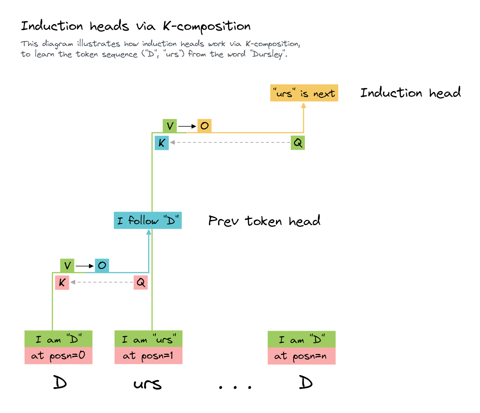
Why is it surprising that induction heads up here? It's surprising because it feels like overkill. The model doesn't care about what token comes after the first copy of the subject, just that it's duplicated. And it already has simpler duplicate token heads. My best guess is that it just already had induction heads around and that, in addition to their main function, they also only activate on duplicated tokens. So it was useful to repurpose this existing machinery.
This suggests that as we look for circuits in larger models life may get more and more complicated, as components in simpler circuits get repurposed and built upon.
First, in the cell below, you should visualise the attention patterns of the induction heads (5.5 and 6.9) on sequences containg repeated tokens, and verify that they are attending to the token after the previous instance of that same token. You might want to repeat code you wrote in the "Validation of duplicate token heads" section.
model.reset_hooks(including_permanent=True)

attn_heads = [(5, 5), (6, 9)]

# Get repeating sequences (note we could also take mean over larger batch)
batch = 1
seq_len = 15
rep_tokens = generate_repeated_tokens(model, seq_len, batch)

# Run cache (we only need attention patterns for layers 5 and 6)
_, cache = model.run_with_cache(
    rep_tokens,
    return_type=None,
    names_filter=lambda name: name.endswith("pattern")
    and any(f".{layer}." in name for layer, head in attn_heads),
)

# Display results
attn = t.stack([cache["pattern", layer][0, head] for (layer, head) in attn_heads])
cv.attention.attention_patterns(
    tokens=model.to_str_tokens(rep_tokens[0]),
    attention=attn,
    attention_head_names=[f"{layer}.{head}" for (layer, head) in attn_heads],
)
One implication of this is that it's useful to categories heads according to whether they occur in simpler circuits, so that as we look for more complex circuits we can easily look for them. This is Hooked to do here! An interesting fact about induction heads is that they work on a sequence of repeated random tokens - notable for being wildly off distribution from the natural language GPT-2 was trained on. Being able to predict a model's behaviour off distribution is a good mark of success for mechanistic interpretability! This is a good sanity check for whether a head is an induction head or not.
We can characterise an induction head by just giving a sequence of random tokens repeated once, and measuring the average attention paid from the second copy of a token to the token after the first copy. At the same time, we can also measure the average attention paid from the second copy of a token to the first copy of the token, which is the attention that the induction head would pay if it were a duplicate token head, and the average attention paid to the previous token to find previous token heads.
Note that this is a superficial study of whether something is an induction head - we totally ignore the question of whether it actually does boost the correct token or whether it composes with a single previous head and how. In particular, we sometimes get anti-induction heads which suppress the induction-y token (no clue why!), and this technique will find those too.
Exercise - validate prev token heads via patching
The paper mentions that heads 2.2 and 4.11 are previous token heads. Hopefully you already validated this in the previous section by plotting the previous token scores (in your replication of Figure 18). But this time, you'll perform a particular kind of path patching to prove that these heads are functioning as previous token heads, in the way implied by our circuit diagram.
Question - what kind of path patching should you perform?
To show these heads are acting as prev token heads in an induction circuit, we want to perform key-patching (i.e. patch the path from the output of the prev token heads to the key inputs of the induction heads).
We expect this to worsen performance, because it interrupts the duplicate token signal provided by the induction heads.
model.reset_hooks(including_permanent=True)

# YOUR CODE HERE - create `induction_head_key_path_patching_results`


imshow(
    100 * induction_head_key_path_patching_results,
    title="Direct effect on Induction Heads' keys",
    labels={"x": "Head", "y": "Layer", "color": "Logit diff.<br>variation"},
    coloraxis=dict(colorbar_ticksuffix="%"),
    width=600,
)
Click to see the expected output
Solution
model.reset_hooks(including_permanent=True)
induction_head_key_path_patching_results = get_path_patch_head_to_heads(
    receiver_heads=[(5, 5), (6, 9)], receiver_input="k", model=model, patching_metric=ioi_metric_2
)
You might notice that there are two other heads in the induction heads box in the paper's diagram, both in brackets (heads 5.8 and 5.9). Can you try and figure out what these heads are doing, and why they're in brackets?
Hint
Recall the path patching section, where you applied patching from attention heads' outputs to the value inputs to the S-inhibition heads (hopefully replicating figure 4b from the paper). Try patching the keys of the S-inhibition heads instead. Do heads 5.8 and 5.9 stand out here?
Answer
After making the plot suggested in the hint, you should find that patching from 5.8 and 5.9 each have around a 5% negative impact on the logit difference if you patch from them to the S-inhibition heads. We'd like to conclude that these are induction heads, and they're acting to increase the attention paid by end to S2. Unfortunately, they don't seem to be induction heads according to the results of figure 18 in the paper (which we replicated in the section "validation of early heads").
It turns out that they're acting as induction heads on this distribution, but not in general. A simple way we can support this hypothesis is to look at attention patterns (we find that S2 pays attention to S1+1 in both head 5.8 and 5.9).
Aside - a lesson in nonlinearity
In the dropdown above, I claimed that 5.8 and 5.9 were doing induction on this distribution. A more rigorous way to test this would be to path patch to the keys of these heads, and see if either of the previous token heads have a large effect. If they do, this is very strong evidence for induction. However, it turns out that neither of the prev token heads affect the model's IOI performance via their path through the fuzzy induction heads. Does this invalidate our hypothesis?
In fact, no, because of nonlinearity. The two prev token heads 2.2 and 4.11 will be adding onto the logits used to calculate the attention probability from S2 to S1+1, rather than adding onto the probabilities directly. SO it might be the case that one head on its own doesn't increase the attention probability very much, both both heads acting together significantly increase it. (Motivating example: suppose we only had 2 possible source tokens, without either head acting the logits are [0.0, -8.0], and the action of each head is to add 4.0 to the second logit. If one head acts then the probability on the second token goes from basically zero to 0.018 (which will have a very small impact on the attention head's output), but if both heads are acting then the logits are equal and the probability is 0.5 (which obviously has a much larger effect)).
This is in fact what I found here - after modifying the path patching function to allow more than one sender head, I found that patching from both 2.2 and 4.11 to 5.8 and 5.9 had a larger effect on the model's IOI performance than patching from either head alone (about a 1% drop in performance for both vs almost 0% for either individually). The same effect can be found when we patch from these heads to all four induction heads, although it's even more pronounced (a 3% and 15% drop respectively for the heads individually, vs 31% for both).
Backup name mover heads
Another fascinating anomaly is that of the backup name mover heads. A standard technique to apply when interpreting model internals is ablations, or knock-out. If we run the model but intervene to set a specific head to zero, what happens? If the model is robust to this intervention, then naively we can be confident that the head is not doing anything important, and conversely if the model is much worse at the task this suggests that head was important. There are several conceptual flaws with this approach, making the evidence only suggestive, e.g. that the average output of the head may be far from zero and so the knockout may send it far from expected activations, breaking internals on any task. But it's still an Hooked technique to apply to give some data.
But a wild finding in the paper is that models have built in redundancy. If we knock out one of the name movers, then there are some backup name movers in later layers that change their behaviour and do (some of) the job of the original name mover head. This means that naive knock-out will significantly underestimate the importance of the name movers.
Let's test this! Let's ablate the most important name mover (which is 9.9, as the code below verifies for us) on just the end token, and compare performance.
model.reset_hooks(including_permanent=True)

ioi_logits, ioi_cache = model.run_with_cache(ioi_dataset.toks)
original_average_logit_diff = logits_to_ave_logit_diff_2(ioi_logits)

s_unembeddings = model.W_U.T[ioi_dataset.s_tokenIDs]
io_unembeddings = model.W_U.T[ioi_dataset.io_tokenIDs]
logit_diff_directions = io_unembeddings - s_unembeddings  # [batch d_model]

per_head_residual, labels = ioi_cache.stack_head_results(layer=-1, return_labels=True)
per_head_residual = einops.rearrange(
    per_head_residual[
        :, t.arange(len(ioi_dataset)).to(device), ioi_dataset.word_idx["end"].to(device)
    ],
    "(layer head) batch d_model -> layer head batch d_model",
    layer=model.cfg.n_layers,
)

per_head_logit_diffs = residual_stack_to_logit_diff(
    per_head_residual, ioi_cache, logit_diff_directions
)

top_layer, top_head = topk_of_Nd_tensor(per_head_logit_diffs, k=1)[0]
print(f"Top Name Mover to ablate: {top_layer}.{top_head}")

# Getting means we can use to ablate
abc_means = ioi_circuit_extraction.compute_means_by_template(abc_dataset, model)[top_layer]


# Define hook function and add to model
def ablate_top_head_hook(z: Float[Tensor, "batch pos head_index d_head"], hook):
    """
    Ablates hook by patching in results
    """
    z[range(len(ioi_dataset)), ioi_dataset.word_idx["end"], top_head] = abc_means[
        range(len(ioi_dataset)), ioi_dataset.word_idx["end"], top_head
    ]
    return z


model.add_hook(utils.get_act_name("z", top_layer), ablate_top_head_hook)

# Run the model, temporarily adds caching hooks and then removes *all* hooks after running,
# including the ablation hook.
ablated_logits, ablated_cache = model.run_with_cache(ioi_dataset.toks)
rprint(
    "\n".join(
        [
            f"{original_average_logit_diff:.4f} = Original logit diff",
            f"{per_head_logit_diffs[top_layer, top_head]:.4f} = Direct Logit Attribution of top name mover head",
            f"{original_average_logit_diff - per_head_logit_diffs[top_layer, top_head]:.4f} = Naive prediction of post ablation logit diff",
            f"{logits_to_ave_logit_diff_2(ablated_logits):.4f} = Logit diff after ablating L{top_layer}H{top_head}",
        ]
    )
)
Top Name Mover to ablate: 9.9

2.8052 = Original logit diff
1.7086 = Direct Logit Attribution of top name mover head
1.0966 = Naive prediction of post ablation logit diff
2.6290 = Logit diff after ablating L9H9
What's going on here? We calculate the logit diff for our full model, and how much of that is coming directly from head 9.9. Given this, we come up with an estimate for what the logit diff will fall to when we ablate this head. In fact, performance is much better than this naive prediction.
Why is this happening? As before, we can look at the direct logit attribution of each head to get a sense of what's going on.
per_head_ablated_residual, labels = ablated_cache.stack_head_results(layer=-1, return_labels=True)
per_head_ablated_residual = einops.rearrange(
    per_head_ablated_residual[
        :, t.arange(len(ioi_dataset)).to(device), ioi_dataset.word_idx["end"].to(device)
    ],
    "(layer head) batch d_model -> layer head batch d_model",
    layer=model.cfg.n_layers,
)
per_head_ablated_logit_diffs = residual_stack_to_logit_diff(
    per_head_ablated_residual, ablated_cache, logit_diff_directions
)
per_head_ablated_logit_diffs = per_head_ablated_logit_diffs.reshape(
    model.cfg.n_layers, model.cfg.n_heads
)


imshow(
    t.stack(
        [
            per_head_logit_diffs,
            per_head_ablated_logit_diffs,
            per_head_ablated_logit_diffs - per_head_logit_diffs,
        ]
    ),
    title="Direct logit contribution by head, pre / post ablation",
    labels={"x": "Head", "y": "Layer"},
    facet_col=0,
    facet_labels=["No ablation", "9.9 is ablated", "Change in head contribution post-ablation"],
    width=1200,
)

scatter(
    y=per_head_logit_diffs.flatten(),
    x=per_head_ablated_logit_diffs.flatten(),
    hover_name=labels,
    range_x=(-1, 1),
    range_y=(-2, 2),
    labels={"x": "Ablated", "y": "Original"},
    title="Original vs Post-Ablation Direct Logit Attribution of Heads",
    width=600,
    add_line="y=x",
)
Click to see the expected output
The first plots show us that, after we ablate head 9.9, while its direct contribution to the logit diff falls (obviously), a lot of contributions from other heads (particularly in layer 10) actually increase. The second plot shows this in a different way (the distinctive heads in the right hand heatmap are the same as the heads lying well below the y=x line in the scatter plot).
One natural hypothesis is that this is because the final LayerNorm scaling has changed, which can scale up or down the final residual stream. This is slightly true, and we can see that the typical head is a bit off from the x=y line. But the average LN scaling ratio is 1.04, and this should uniformly change all heads by the same factor, so this can't be sufficient.
ln_scaling_no_ablation = ioi_cache["ln_final.hook_scale"][
    t.arange(len(ioi_dataset)), ioi_dataset.word_idx["end"]
].squeeze()
ln_scaling_ablated = ablated_cache["ln_final.hook_scale"][
    t.arange(len(ioi_dataset)), ioi_dataset.word_idx["end"]
].squeeze()

scatter(
    y=ln_scaling_ablated,
    x=ln_scaling_no_ablation,
    labels={"x": "No ablation", "y": "Ablation"},
    title=f"Final LN scaling factors compared (ablation vs no ablation)<br>Average ratio = {(ln_scaling_no_ablation / ln_scaling_ablated).mean():.4f}",
    width=700,
    add_line="y=x",
)
Click to see the expected output
Exercise to the reader: Can you finish off this analysis? What's going on here? Why are the backup name movers changing their behaviour? Why is one negative name mover becoming significantly less important?
Positional vs token information being moved
In section A of the appendix (titled Disentangling token and positional signal in the output of S-Inhibition Heads), the authors attempt to figure out whether the S-Inhibition heads are using token or positional information to supress the attention paid to S1. This is illustrated in my IOI diagram, by purple vs pink boxes.
The way the authors find out which one is which is ingenious. They construct datasets from the original IOI dataset, with some of the signals erased or flipped. For instance, if they want to examine the effect of inverting the positional information but preserving the token information written by the S-inhibition heads, they can replace sentences like:
When Mary and John went to the store, John gave a drink to Mary
with:
When John and Mary went to the store, John gave a drink to Mary
Let's be exactly clear on why this works. The information written to the end token position by the S-inhibition heads will be some combination of "don't pay attention to the duplicated token" and "don't pay attention to the token that's in the same position as the duplicated token". If we run our model on the first sentence above but then patch in the second sentence, then:
- The "don't pay attention to the duplicated token" signal will be unchanged (because this signal still refers to John)
- The "don't pay attention to the token that's in the same position as the duplicated token" signal will flip (because this information points to the position of
Maryin the second sentence, hence to the position ofJohnin the first sentence).
That was just one example (flipping positional information, keeping token information the same), but we can do any of six different types of flip:
| Token signal | Positional signal | Sentence | ABB -> ? |
|---|---|---|---|
| Same | Same | When Mary and John went to the store, John gave a drink to Mary |
ABB |
| Random | Same | When Emma and Paul went to the store, Paul gave ... |
CDD |
| Inverted | Same | When John and Mary went to the store, Mary gave ... |
BAA |
| Same | Inverted | When John and Mary went to the store, John gave ... |
BAB |
| Random | Inverted | When Paul and Emma went to the store, Emma gave ... |
DCD |
| Inverted | Inverted | When Mary and John went to the store, Mary gave ... |
ABA |
We use the gen_flipped_prompts method to generate each of these datasets:
datasets: list[tuple[tuple, str, IOIDataset]] = [
    ((0, 0), "original", ioi_dataset),
    ((1, 0), "random token", ioi_dataset.gen_flipped_prompts("ABB->CDD, BAB->DCD")),
    ((2, 0), "inverted token", ioi_dataset.gen_flipped_prompts("ABB->BAA, BAB->ABA")),
    ((0, 1), "inverted position", ioi_dataset.gen_flipped_prompts("ABB->BAB, BAB->ABB")),
    (
        (1, 1),
        "inverted position, random token",
        ioi_dataset.gen_flipped_prompts("ABB->DCD, BAB->CDD"),
    ),
    (
        (2, 1),
        "inverted position, inverted token",
        ioi_dataset.gen_flipped_prompts("ABB->ABA, BAB->BAA"),
    ),
]

results = t.zeros(3, 2).to(device)

s2_inhibition_heads = CIRCUIT["s2 inhibition"]
layers = set(layer for layer, head in s2_inhibition_heads)

names_filter = lambda name: name in [utils.get_act_name("z", layer) for layer in layers]


def patching_hook_fn(
    z: Float[Tensor, "batch seq head d_head"], hook: HookPoint, cache: ActivationCache
):
    heads_to_patch = [head for layer, head in s2_inhibition_heads if layer == hook.layer()]
    z[:, :, heads_to_patch] = cache[hook.name][:, :, heads_to_patch]
    return z


for (row, col), desc, dataset in datasets:
    # Get cache of values from the modified dataset
    _, cache_for_patching = model.run_with_cache(
        dataset.toks, names_filter=names_filter, return_type=None
    )

    # Run model on IOI dataset, but patch S-inhibition heads with signals from modified dataset
    patched_logits = model.run_with_hooks(
        ioi_dataset.toks,
        fwd_hooks=[(names_filter, partial(patching_hook_fn, cache=cache_for_patching))],
    )

    # Get logit diff for patched results
    # Note, we still use IOI dataset for our "correct answers" reference point
    results[row, col] = logits_to_ave_logit_diff_2(patched_logits, ioi_dataset)


imshow(
    results,
    labels={"x": "Positional signal", "y": "Token signal"},
    x=["Original", "Inverted"],
    y=["Original", "Random", "Inverted"],
    title="Logit diff after changing all S2 inhibition heads' output signals via patching",
    text_auto=".2f",
    width=700,
)
Click to see the expected output
What are your interpretations of this plot?
Some thoughts
A few sanity checks, which are what we'd expect from this plot (and hence validate our code as probably being correct):
When token and positional signals are inverted, performance is close to negative of the original performance. Inverting the positional signal makes performance worse. Randomizing the token signal makes performance worse. Inverting the token signal makes performance worse. This effect is larger than randomizing (because we're pointing away from a correct answer, rather than just in a random direction).There are two main interesting findings from this plot (which we might have guessed at beforehand, but couldn't have been certain about):
The row and column differences are close to constant (column diff is approx 4.5, row diff is approx 0.75). In other words, the logit diff can be well approximated by a linear combination of the positional and token signal correlations (where correlation is 1 if the signal points towards the correct value, -1 if it points away, and 0 if it points in a random direction).
The coefficients on the positional signal correlation is much bigger than the coefficient on the token signal correlation. The former is about 4.5, the latter is about 1.5. This tells us that positional information is a lot more important than token information.
* One possible intuition here is that name information (i.e. representing the identity of the token " John") takes up many dimensions, so is probably harder for the model. Relative positional information on the other hand will mostly have fewer dimensions. Since the model only needs to move enough information to single out a single positional index from about 15-20, rather than single out a name in the entire set of names. This is jus a guess though, and I'd love to hear other interpretations.
Let's dig a little deeper. Rather than just looking at the S-inhibition heads collectively, we can look at each of them individually.
Exercise - decompose S-Inhibition heads
Make the same plot as above, but after intervening on each of the S-inhibition heads individually.
You can do this by creating a results tensor of shape (M, 3, 2) where M is the number of S-inhibition heads, and each slice contains the results of intervening on that particular head. We've given you the code to plot your results below, all you need to do is fill in results.
(Note - we recommend computing the results as (logit_diff - clean_logit_diff) / clean_logit_diff, so your baseline is 0 for "this patching has no effect" and -1 for "this patching completely destroys model performance", to make the plot look clearer.)
results = t.zeros(len(CIRCUIT["s2 inhibition"]), 3, 2).to(device)


YOUR CODE HERE - fill in the `results` tensor!

    imshow(
        (results - results[0, 0, 0]) / results[0, 0, 0],
        labels={"x": "Positional signal", "y": "Token signal"},
        x=["Original", "Inverted"],
        y=["Original", "Random", "Inverted"],
        title="Logit diff after patching individual S2 inhibition heads (as proportion of clean logit diff)",
        facet_col=0,
        facet_labels=[f"{layer}.{head}" for (layer, head) in CIRCUIT["s2 inhibition"]],
        facet_col_spacing=0.08,
        width=1100,
        text_auto=".2f",
    )
Click to see the expected output
Solution
results = t.zeros(len(CIRCUIT["s2 inhibition"]), 3, 2).to(device)
def patching_hook_fn(
    z: Float[Tensor, "batch seq head d_head"], hook: HookPoint, cache: ActivationCache, head: int
):
    z[:, :, head] = cache[hook.name][:, :, head]
    return z
for i, (layer, head) in enumerate(CIRCUIT["s2 inhibition"]):
    model.reset_hooks(including_permanent=True)
hook_name = utils.get_act_name("z", layer)
for (row, col), desc, dataset in datasets:
        # Get cache of values from the modified dataset
        _, cache_for_patching = model.run_with_cache(
            dataset.toks, names_filter=lambda name: name == hook_name, return_type=None
        )
# Run model on IOI dataset, but patch S-inhibition heads with modified dataset signals
        patched_logits = model.run_with_hooks(
            ioi_dataset.toks,
            fwd_hooks=[
                (hook_name, partial(patching_hook_fn, cache=cache_for_patching, head=head))
            ],
        )
# Get logit diff for patched results
        # Note, we still use IOI dataset for our "correct answers" reference point
        results[i, row, col] = logits_to_ave_logit_diff_2(patched_logits, ioi_dataset)
imshow(
    (results - results[0, 0, 0]) / results[0, 0, 0],
    labels={"x": "Positional signal", "y": "Token signal"},
    x=["Original", "Inverted"],
    y=["Original", "Random", "Inverted"],
    title="Logit diff after patching individual S2 inhibition heads (as proportion of clean logit diff)",
    facet_col=0,
    facet_labels=[f"{layer}.{head}" for (layer, head) in CIRCUIT["s2 inhibition"]],
    facet_col_spacing=0.08,
    width=1100,
    text_auto=".2f",
)
Noteworthy features of this plot:
- Every head cares more about positional signal than token signal
- Head
8.6(the biggest S-inhibition head) cares MUCH more about positional signal, in fact it doesn't care at all about token signal- Suggests maybe
8.6was the first head which learned to do this task, and subsequent heads basically just helped out by providing the remainder (which was token signal). Shows the heads specialise.
- Suggests maybe
- The only heads that kinda care about token signal are
7.9and8.10(but they still both care about positional signal almost twice as much) - The approximation of logit diff as a sum of positional and token signal correlations still seems to hold for each head individually, although the coefficients for each head are different.
Further Reading
Here is a collection of links for further reading, which haven't already been mentioned:
- Some Lessons Learned from Studying Indirect Object Identification in GPT-2 small
- A blog post by the authors of this paper, which goes into more detail about the experiments and results.
- Causal Scrubbing: a method for rigorously testing interpretability hypotheses [Redwood Research]
- Introduces the idea of causal scubbing, a proposed systematic method for evaluting the quality of mechanistic interpretations
Suggested topics for further exploration
Here are some future directions, some suggested by Neel, others by the authors of the paper. Many of these might make good capstone projects!
- 3 letter acronyms (or more!)
- Converting names to emails.
- An extension task is e.g. constructing an email from a snippet like the following: Name: Neel Nanda; Email: last name dot first name k @ gmail
- Grammatical rules
- Learning that words after full stops are capital letters
- Verb conjugation
- Choosing the right pronouns (e.g. he vs she vs it vs they)
- Whether something is a proper noun or not
- Detecting sentiment (e.g. predicting whether something will be described as good vs bad)
- Interpreting memorisation. E.g., there are times when GPT-2 knows surprising facts like people’s contact information. How does that happen?
- Counting objects described in text. E.g.: I picked up an apple, a pear, and an orange. I was holding three fruits.
- Extensions from Alex Variengien
- Understanding what's happening in the adversarial examples: most notably S-Inhibition Head attention pattern (hard). (S-Inhibition heads are mentioned in the IOI paper)
- Understanding how are positional signal encoded (relative distance, something else?) bonus point if we have a story that include the positional embeddings and that explain how the difference between position is computed (if relative is the right framework) by Duplicate Token Heads / Induction Heads. (hard, but less context dependant)
- What are the role of MLPs in IOI (quite broad and hard)
- What is the role of Duplicate Token Heads outside IOI? Are they used in other Q-compositions with S-Inhibition Heads? Can we describe how their QK circuit implement "collision detection" at a parameter level? (Last question is low context dependant and quite tractable)
- What is the role of Negative/ Backup/ regular Name Movers Heads outside IOI? Can we find examples on which Negative Name Movers contribute positively to the next-token prediction?
- What are the differences between the 5 inductions heads present in GPT2-small? What are the heads they rely on / what are the later heads they compose with (low context dependence form IOI)
- Understanding 4.11, (a really sharp previous token heads) at the parameter level. I think this can be quite tractable given that its attention pattern is almost perfectly off-diagonal
- What are the conditions for compensation mechanisms to occur? Is it due to drop-out? (Arthur Conmy is working on this - feel free to reach out to arthur@rdwrs.com )
- Extensions from Arthur Conmy
- Understand IOI in GPT-Neo: it's a same size model but does IOI via composition of MLPs
- Understand IOI in the Stanford mistral models - they all seem to do IOI in the same way, so maybe look at the development of the circuit through training?
- Help out Redwood Research’s interpretability team by finding heuristics implemented by GPT-2 small
- This LessWrong post from 6 months ago outlines some features of the IOI task that made it a good choice to study, and suggests other tasks that might meet these criteria / how you might go about finding such tasks.
Suggested paper replications
A circuit for Python docstrings in a 4-layer attention-only transformer
This work was produced as part of the SERI ML Alignment Theory Scholars Program (Winter 2022) under the supervision of Neel Nanda. Similar to how the IOI paper searched for in some sense the simplest kind of circuit which required 3 layers, this work was looking for the simplest kind of circuit which required 4 layers. The task they investigated was the docstring task - can you predict parameters in the right order, in situations like this:
def port(self, load, size, files, last):
    '''oil column piece

    :param load: crime population
    :param size: unit dark
    :param
The token that follows should be files, and just like in the case of IOI we can deeply analyze how the transformer solves this task. Unlike IOI, we're looking at a 4-layer transformer which was trained on code (not GPT2-Small), which makes a lot of the analysis cleaner (even though the circuit has more levels of composition than IOI does).
For an extra challenge, rather than replicating the authors' results, you can try and perform this investigation yourself, without seeing what tools the authors of the paper used! Most will be similar to the ones you've used in the exercises so far.
This might be a good replication for you if:
- You enjoyed most/all sections of these exercises, and want to practice using the tools you learned in a different context
- You don't want to try anything too far left field from the content of these exercises (this post also comes with a Colab notebook which can be referred to if you're stuck)
Mechanistically interpreting time in GPT-2 small
This work was done by a group of independent researchers, supervised by Arthur Conmy. The task was to interpret how GPT2-Small can solve the task of next day prediction, i.e. predicting the next token in sentences like If today is Monday, tomorrow is. This replication is easier than the previous one, since the core circuit only contains one attention head rather than a composition of several. For this reason, we'd more strongly encourage trying to do this replication without guidance, i.e. have a crack at it before reading the full post.
How does GPT-2 compute greater-than? Interpreting mathematical abilities in a pre-trained language model
This paper came out of the REMIX program run by Redwood Research. It analyses a circuit in GPT2-Small, much like this one. Here, the circuit is for computing greater-than; in other words detecting that sentences like The war lasted from the year 1732 to the year 17... will be completed by valid two-digit end years (years > 32). The paper identifies a circuit, explains the role of each circuit component, and also finds related tasks that activate the circuit.
For an extra challenge, rather than replicating this paper, you can try and perform this investigation yourself, without seeing what tools the authors of the paper used! Many will be similar to the ones you've used in the exercises so far; some will be different. In particular, there will be some analysis of individual neurons in this replication, unlike in this IOI notebook.
This might be a good replication for you if:
- You enjoyed most/all sections of these exercises, and want to practice using the tools you learned in a different context
- You don't want to try anything too far left field from the content of these exercises (although this is probably more challenging than the docstring circuit, mainly due to the presence of MLPs)
Towards Automated Circuit Discovery for Mechanistic Interpretability / Attribution Patching Outperforms Automated Circuit Discovery
These two are grouped together, because they both study the possibility of scaling circuit discovery tools using automation. Automated Circuit Discovery (ACDC) was a tool discovered by Arthur Conmy & collaborators partially done at Redwood Research. They automate several of the techniques we've used in these exercises (in particular activation & patch patching), iteratively severing connections between components until we're left with a minimal circuit which can still effectively solve the task. Attribution patching is slightly different; it approximates the effect of each component on the model's output (and by extension its importance in a particular task) by a simple and computationally cheap first-order approximation.
Either of these techniques would serve as suitable replication challenges over the course of a week. There's also a lot of work that can still be done in improving or refining these techniques.
This might be a good replication for you if:
- You enjoyed the exercises in this section, in particular those on activation and path patching
- You're looking for a project which is more focused on coding and implementation than on theory
- You're excited about exploring ways to scale / automate circuit discovery efficiently