3️⃣ Activation Patching

Learning Objectives

• Understand the idea of activation patching, and how it can be used
  • Implement some of the activation patching helper functinos in transformerlens from scratch (i.e. using hooks)
• Use activation patching to track the layers & sequence positions in the residual stream where important information is stored and processed
• By the end of this section, you should be able to draw a rough sketch of the IOI circuit

Introduction

The obvious limitation to the techniques used above is that they only look at the very end of the circuit - the parts that directly affect the logits. Clearly this is not sufficient to understand the circuit! We want to understand how things compose together to produce this final output, and ideally to produce an end-to-end circuit fully explaining this behaviour.

The technique we'll use to investigate this is called activation patching. This was first introduced in David Bau and Kevin Meng's excellent ROME paper, there called causal tracing.

The setup of activation patching is to take two runs of the model on two different inputs, the clean run and the corrupted run. The clean run outputs the correct answer and the corrupted run does not. The key idea is that we give the model the corrupted input, but then intervene on a specific activation and patch in the corresponding activation from the clean run (ie replace the corrupted activation with the clean activation), and then continue the run. And we then measure how much the output has updated towards the correct answer.

We can then iterate over many possible activations and look at how much they affect the corrupted run. If patching in an activation significantly increases the probability of the correct answer, this allows us to localise which activations matter.

In other words, this is a noising algorithm (unlike last section which was mostly denoising).

The ability to localise is a key move in mechanistic interpretability - if the computation is diffuse and spread across the entire model, it is likely much harder to form a clean mechanistic story for what's going on. But if we can identify precisely which parts of the model matter, we can then zoom in and determine what they represent and how they connect up with each other, and ultimately reverse engineer the underlying circuit that they represent.

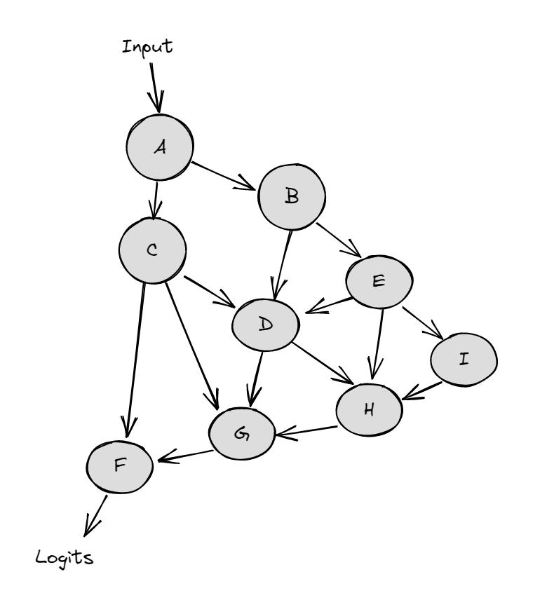
The diagrams below demonstrate activation patching on an abstract neural network (the nodes represent activations, and the arrows between them are weight connections).

A regular forward pass on the clean input looks like:

And activation patching from a corrupted input (green) into a forward pass for the clean input (black) looks like:

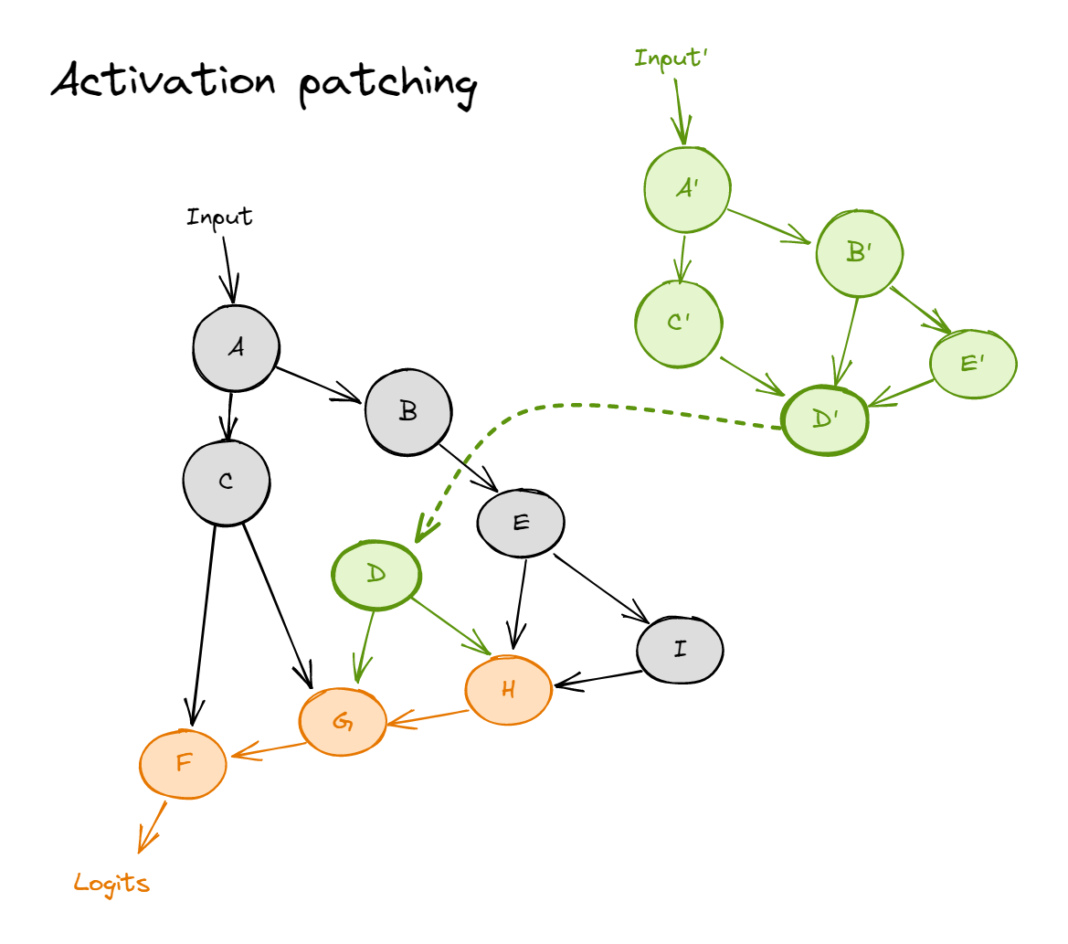
where the dotted line represents patching in a value (i.e. during the forward pass on the clean input, we replace node $D$ with the value it takes on the corrupted input). Nodes $H$, $G$ and $F$ are colored orange, to represent that they now follow a distribution which is not the same as clean or corrupted.

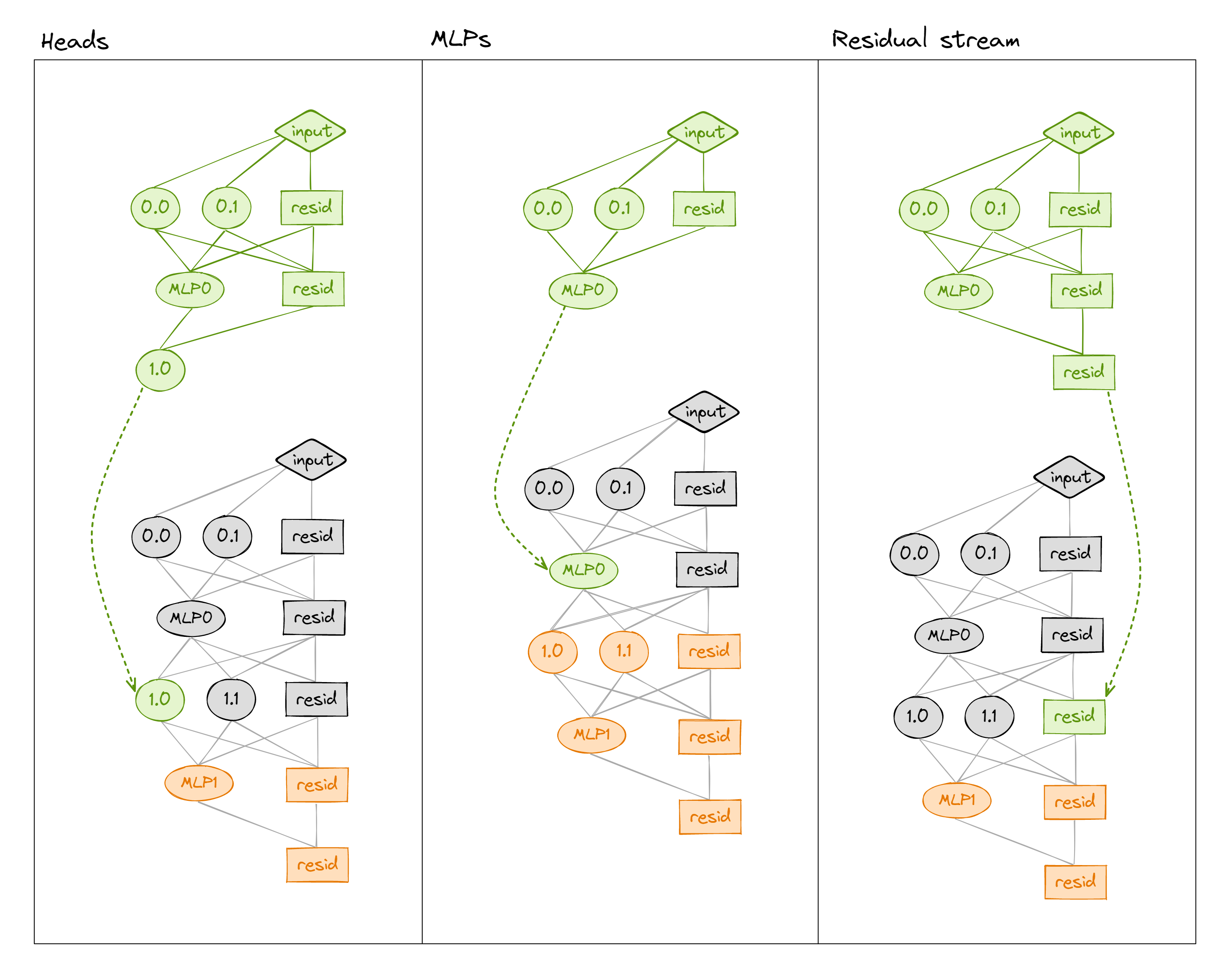
We can patch into a transformer in many different ways (e.g. values of the residual stream, the MLP, or attention heads' output - see below). We can also get even more granular by patching at particular sequence positions (not shown in diagram).

Noising vs denoising

We might call this algorithm a type of noising, since we're running the model on a clean input and adding noise by patching in from the corrupted input. We can also consider the opposite algorithm, denoising, where we run the model on a corrupted input and remove noise by patching in from the clean input.

When would you use noising vs denoising? It depends on your goals. The results of denoising are much stronger, because showing that a component or set of components is sufficient for a task is a big deal. On the other hand, the complexity of transformers and interdependence of components means that noising a model can have unpredictable consequences. If loss goes up when we ablate a component, it doesn't necessarily mean that this component was necessary for the task. As an example, ablating MLP0 in gpt2-small seems to make performance much worse on basically any task (because it acts as a kind of extended embedding; more on this later in these exercises), but it's not doing anything important which is specfic for the IOI task.

Example: denoising the residual stream

The above was all fairly abstract, so let's zoom in and lay out a concrete example to understand Indirect Object Identification. We'll start with an exercise on denoising, but we'll move onto noising later in this section (and the next section, on path patching).

Here our clean input will be the original sentences (e.g. "When Mary and John went to the store, John gave a drink to") and our corrupted input will have the subject token flipped (e.g. "When Mary and John went to the store, Mary gave a drink to"). Patching by replacing corrupted residual stream values with clean values is a causal intervention which will allow us to understand precisely which parts of the network are identifying the indirect object. If a component is important, then patching in (replacing that component's corrupted output with its clean output) will reverse the signal that this component produces, hence making performance much better.

Note - the noising and denoising terminology doesn't exactly fit here, since the "noised dataset" actually reverses the signal rather than erasing it. The reason we're describing this as denoising is more a matter of framing - we're trying to figure out which components / activations are sufficient to recover performance, rather than which are necessary. If you're ever confused, this is a useful framing to have - noising tells you what is necessary, denoising tells you what is sufficient.

Question - we could instead have our corrupted sentence be "When John and Mary went to the store, Mary gave a drink to" (i.e. flip all 3 occurrences of names in the sentence). Why do you think we don't do this?

One natural thing to patch in is the residual stream at a specific layer and specific position. For example, the model is likely intitially doing some processing on the S2 token to realise that it's a duplicate, but then uses attention to move that information to the end token. So patching in the residual stream at the end token will likely matter a lot in later layers but not at all in early layers.

We can zoom in much further and patch in specific activations from specific layers. For example, we think that the output of head 9.9 on the final token is significant for directly connecting to the logits, so we predict that just patching the output of this head will significantly affect performance.

Note that this technique does not tell us how the components of the circuit connect up, just what they are.

TransformerLens has helpful built-in functions to perform activation patching, but in order to understand the process better, you're now going to implement some of these functions from first principles (i.e. just using hooks). You'll be able to test your functions by comparing their output to the built-in functions.

If you need a refresher on hooks, you can return to the exercises on induction heads (which take you through how to use hooks, as well as how to cache activations).

from transformer_lens import patching

Creating a metric

Before we patch, we need to create a metric for evaluating a set of logits. Since we'll be running our corrupted prompts (with S2 replaced with the wrong name) and patching in our clean prompts, it makes sense to choose a metric such that:

• A value of zero means no change (from the performance on the corrupted prompt)
• A value of one means clean performance has been completely recovered

For example, if we patched in the entire clean prompt, we'd get a value of one. If our patching actually makes the model even better at solving the task than its regular behaviour on the clean prompt then we'd get a value greater than 1, but generally we expect values between 0 and 1.

It also makes sense to have the metric be a linear function of the logit difference. This is enough to uniquely specify a metric.

clean_tokens = tokens
# Swap each adjacent pair to get corrupted tokens
indices = [i + 1 if i % 2 == 0 else i - 1 for i in range(len(tokens))]
corrupted_tokens = clean_tokens[indices]

print(
    "Clean string 0:    ",
    model.to_string(clean_tokens[0]),
    "\nCorrupted string 0:",
    model.to_string(corrupted_tokens[0]),
)

clean_logits, clean_cache = model.run_with_cache(clean_tokens)
corrupted_logits, corrupted_cache = model.run_with_cache(corrupted_tokens)

clean_logit_diff = logits_to_ave_logit_diff(clean_logits, answer_tokens)
print(f"Clean logit diff: {clean_logit_diff:.4f}")

corrupted_logit_diff = logits_to_ave_logit_diff(corrupted_logits, answer_tokens)
print(f"Corrupted logit diff: {corrupted_logit_diff:.4f}")

Exercise - create a metric

Fill in the function ioi_metric below, to create the required metric. Note that we can afford to use default arguments in this function, because we'll be using the same dataset for this whole section.

Important note - this function needs to return a scalar tensor, rather than a float. If not, then some of the patching functions later on won't work. The type signature of this is Float[Tensor, ""].

Second important note - we've defined this to be 0 when performance is the same as on corrupted input, and 1 when it's the same as on clean input. This is because we're performing a denoising algorithm; we're looking for activations which are sufficient for recovering a model's performance (i.e. activations which have enough information to recover the correct answer from the corrupted input). Our "null hypothesis" is that the component isn't sufficient, and so patching it by replacing corrupted with clean values doesn't recover any performance. In later sections we'll be doing noising, and we'll define a new metric function for that.

def ioi_metric(
    logits: Float[Tensor, "batch seq d_vocab"],
    answer_tokens: Int[Tensor, "batch 2"] = answer_tokens,
    corrupted_logit_diff: float = corrupted_logit_diff,
    clean_logit_diff: float = clean_logit_diff,
) -> Float[Tensor, ""]:
    """
    Linear function of logit diff, calibrated so that it equals 0 when performance is same as on
    corrupted input, and 1 when performance is same as on clean input.
    """
    raise NotImplementedError()


t.testing.assert_close(ioi_metric(clean_logits).item(), 1.0)
t.testing.assert_close(ioi_metric(corrupted_logits).item(), 0.0)
t.testing.assert_close(ioi_metric((clean_logits + corrupted_logits) / 2).item(), 0.5)

def ioi_metric(
    logits: Float[Tensor, "batch seq d_vocab"],
    answer_tokens: Int[Tensor, "batch 2"] = answer_tokens,
    corrupted_logit_diff: float = corrupted_logit_diff,
    clean_logit_diff: float = clean_logit_diff,
) -> Float[Tensor, ""]:
    """
    Linear function of logit diff, calibrated so that it equals 0 when performance is same as on
    corrupted input, and 1 when performance is same as on clean input.
    """
    patched_logit_diff = logits_to_ave_logit_diff(logits, answer_tokens)
    return (patched_logit_diff - corrupted_logit_diff) / (clean_logit_diff - corrupted_logit_diff)
t.testing.assert_close(ioi_metric(clean_logits).item(), 1.0)
t.testing.assert_close(ioi_metric(corrupted_logits).item(), 0.0)
t.testing.assert_close(ioi_metric((clean_logits + corrupted_logits) / 2).item(), 0.5)

Residual Stream Patching

Lets begin with a simple example: we patch in the residual stream at the start of each layer and for each token position. Before you write your own function to do this, let's see what this looks like with TransformerLens' patching module. Run the code below.

act_patch_resid_pre = patching.get_act_patch_resid_pre(
    model=model,
    corrupted_tokens=corrupted_tokens,
    clean_cache=clean_cache,
    patching_metric=ioi_metric,
)

labels = [f"{tok} {i}" for i, tok in enumerate(model.to_str_tokens(clean_tokens[0]))]

imshow(
    act_patch_resid_pre,
    labels={"x": "Position", "y": "Layer"},
    x=labels,
    title="resid_pre Activation Patching",
    width=700,
)

Question - what is the interpretation of this graph? What significant things does it tell you about the nature of how the model solves this task?

Exercise - implement head-to-residual patching

Now, you should implement the get_act_patch_resid_pre function below, which should give you results just like the code you ran above. A quick refresher on how to use hooks in this way:

• Hook functions take arguments tensor: torch.Tensor and hook: HookPoint. It's often easier to define a hook function taking more arguments than these, and then use functools.partial when it actually comes time to add your hook.
• The function model.run_with_hooks takes arguments:
  • The tokens to run (as first argument)
  • fwd_hooks - a list of (hook_name, hook_fn) tuples. Remember that you can use utils.get_act_name to get hook names.
• Tip - it's good practice to have model.reset_hooks() at the start of functions which add and run hooks. This is because sometimes hooks fail to be removed (if they cause an error while running). There's nothing more frustrating than fixing a hook error only to get the same error message, not realising that you've failed to clear the broken hook!

def patch_residual_component(
    corrupted_residual_component: Float[Tensor, "batch pos d_model"],
    hook: HookPoint,
    pos: int,
    clean_cache: ActivationCache,
) -> Float[Tensor, "batch pos d_model"]:
    """
    Patches a given sequence position in the residual stream, using the value
    from the clean cache.
    """
    raise NotImplementedError()


def get_act_patch_resid_pre(
    model: HookedTransformer,
    corrupted_tokens: Float[Tensor, "batch pos"],
    clean_cache: ActivationCache,
    patching_metric: Callable[[Float[Tensor, "batch pos d_vocab"]], float],
) -> Float[Tensor, "3 layer pos"]:
    """
    Returns an array of results of patching each position at each layer in the residual
    stream, using the value from the clean cache.

    The results are calculated using the patching_metric function, which should be
    called on the model's logit output.
    """
    raise NotImplementedError()


act_patch_resid_pre_own = get_act_patch_resid_pre(
    model, corrupted_tokens, clean_cache, ioi_metric
)

t.testing.assert_close(act_patch_resid_pre, act_patch_resid_pre_own)

def patch_residual_component(
    corrupted_residual_component: Float[Tensor, "batch pos d_model"],
    hook: HookPoint,
    pos: int,
    clean_cache: ActivationCache,
) -> Float[Tensor, "batch pos d_model"]:
    """
    Patches a given sequence position in the residual stream, using the value
    from the clean cache.
    """
    corrupted_residual_component[:, pos, :] = clean_cache[hook.name][:, pos, :]
    return corrupted_residual_component
def get_act_patch_resid_pre(
    model: HookedTransformer,
    corrupted_tokens: Float[Tensor, "batch pos"],
    clean_cache: ActivationCache,
    patching_metric: Callable[[Float[Tensor, "batch pos d_vocab"]], float],
) -> Float[Tensor, "3 layer pos"]:
    """
    Returns an array of results of patching each position at each layer in the residual
    stream, using the value from the clean cache.
    The results are calculated using the patching_metric function, which should be
    called on the model's logit output.
    """
    model.reset_hooks()
    seq_len = corrupted_tokens.size(1)
    results = t.zeros(model.cfg.n_layers, seq_len, device=device, dtype=t.float32)
for layer in tqdm(range(model.cfg.n_layers)):
        for position in range(seq_len):
            hook_fn = partial(patch_residual_component, pos=position, clean_cache=clean_cache)
            patched_logits = model.run_with_hooks(
                corrupted_tokens,
                fwd_hooks=[(utils.get_act_name("resid_pre", layer), hook_fn)],
            )
            results[layer, position] = patching_metric(patched_logits)
return results

Once you've passed the tests, you can plot your results.

imshow(
    act_patch_resid_pre_own,
    x=labels,
    title="Logit Difference From Patched Residual Stream",
    labels={"x": "Sequence Position", "y": "Layer"},
    width=700,
)

Patching in residual stream by block

Rather than just patching to the residual stream in each layer, we can also patch just after the attention layer or just after the MLP. This gives is a slightly more refined view of which tokens matter and when.

The function patching.get_act_patch_block_every works just like get_act_patch_resid_pre, but rather than just patching to the residual stream, it patches to resid_pre, attn_out and mlp_out, and returns a tensor of shape (3, n_layers, seq_len).

One important thing to note - we're cycling through the resid_pre, attn_out and mlp_out and only patching one of them at a time, rather than patching all three at once.

act_patch_block_every = patching.get_act_patch_block_every(
    model, corrupted_tokens, clean_cache, ioi_metric
)

imshow(
    act_patch_block_every,
    x=labels,
    facet_col=0,  # This argument tells plotly which dimension to split into separate plots
    facet_labels=["Residual Stream", "Attn Output", "MLP Output"],  # Subtitles of separate plots
    title="Logit Difference From Patched Attn Head Output",
    labels={"x": "Sequence Position", "y": "Layer"},
    width=1200,
)

clean_prompt, clean_answer = "The White House is where the", " president" #Note the space in the answer!
corrupted_prompt, corrupted_answer = "The Haunted House is where the", " ghosts"
clean_tokens = model.to_tokens(clean_prompt)
corrupted_tokens = model.to_tokens(corrupted_prompt)
assert clean_tokens.shape == corrupted_tokens.shape, "clean and corrupted tokens must have same shape"
clean_token = model.to_single_token(clean_answer)
corrupted_token = model.to_single_token(corrupted_answer)
utils.test_prompt(clean_prompt, clean_answer, model)
utils.test_prompt(corrupted_prompt, corrupted_answer, model)
clean_logits, clean_cache = model.run_with_cache(clean_tokens)
def answer_metric(
    logits: Float[Tensor, "batch seq d_vocab"],
    clean_token: Int = clean_token,
    corrupted_token: Int = corrupted_token,
) -> Float[Tensor, "batch"]:
    return logits[:, -1, clean_token] - logits[:, -1, corrupted_token]
act_patch_block_every = patching.get_act_patch_block_every(model, corrupted_tokens, clean_cache, answer_metric)
imshow(
    act_patch_block_every,
    x=["<endoftext>","The", "White/Haunted", "House", "is", "where", "the"],
    facet_col=0,  # This argument tells plotly which dimension to split into separate plots
    facet_labels=["Residual Stream", "Attn Output", "MLP Output"],  # Subtitles of separate plots
    title="Logit Difference (president - ghosts)",
    labels={"x": "Sequence Position", "y": "Layer"},
    width=1200,
)

Tied embeddings (what MLP0 is doing)

It's often observed on GPT-2 Small that MLP0 matters a lot, and that ablating it utterly destroys performance. The current accepted hypothesis is that the first MLP layer is essentially acting as an extension of the embedding, and that when later layers want to access the input tokens they mostly read in the output of the first MLP layer, rather than the token embeddings. Within this frame, the first attention layer doesn't do much.

In this framing, it makes sense that MLP0 matters on S2, because that's the one position with a different input token (i.e. it has a different extended embedding between the two prompt versions, and all other tokens will have basically the same extended embeddings).

Why does this happen? It seems like most of the effect comes from the fact that the embedding and unembedding matrices in GPT2-Small are tied, i.e. the one equals the transpose of the other. On one hand this seems principled - if two words mean similar things (e.g. "big" and "large") then they should be substitutable, i.e. have similar embeddings and unembeddings. This would seem to suggest that the geometric structure of the embedding and unembedding spaces should be related. On the other hand, there's one major reason why this isn't as principled as it seems - the embedding and the unembedding together form the direct path (if we had no other components then the transformer would just be the linear map $x \to x^T W_E W_U$), and we do not want this to be symmetric because bigram prediction isn't symmetric! As an example, if $W_E = W_U^T$ then in order to predict "Barack Obama" as a probable bigram, we'd also have to predict "Obama Barack" with equally high probability, which obviously shouldn't happen. So it makes sense that the first MLP layer might be used in part to overcome this asymmetry: we now think of $\operatorname{MLP}_0(x^T W_E) W_U$ as the direct path, which is no longer symmetric when $W_E$ and $W_U$ are tied.

Exercise (optional) - implement head-to-block patching

If you want, you can implement the get_act_patch_resid_pre function for fun, although it's similar enough to the previous exercise that doing this isn't compulsory.

def get_act_patch_block_every(
    model: HookedTransformer,
    corrupted_tokens: Float[Tensor, "batch pos"],
    clean_cache: ActivationCache,
    patching_metric: Callable[[Float[Tensor, "batch pos d_vocab"]], float],
) -> Float[Tensor, "3 layer pos"]:
    """
    Returns an array of results of patching each position at each layer in the residual stream,
    using the value from the clean cache.

    The results are calculated using the patching_metric function, which should be called on the
    model's logit output.
    """
    raise NotImplementedError()


act_patch_block_every_own = get_act_patch_block_every(
    model, corrupted_tokens, clean_cache, ioi_metric
)

t.testing.assert_close(act_patch_block_every, act_patch_block_every_own)

imshow(
    act_patch_block_every_own,
    x=labels,
    facet_col=0,
    facet_labels=["Residual Stream", "Attn Output", "MLP Output"],
    title="Logit Difference From Patched Attn Head Output",
    labels={"x": "Sequence Position", "y": "Layer"},
    width=1200,
)

def get_act_patch_block_every(
    model: HookedTransformer,
    corrupted_tokens: Float[Tensor, "batch pos"],
    clean_cache: ActivationCache,
    patching_metric: Callable[[Float[Tensor, "batch pos d_vocab"]], float],
) -> Float[Tensor, "3 layer pos"]:
    """
    Returns an array of results of patching each position at each layer in the residual stream,
    using the value from the clean cache.
    The results are calculated using the patching_metric function, which should be called on the
    model's logit output.
    """
    model.reset_hooks()
    results = t.zeros(3, model.cfg.n_layers, tokens.size(1), device=device, dtype=t.float32)
for component_idx, component in enumerate(["resid_pre", "attn_out", "mlp_out"]):
        for layer in tqdm(range(model.cfg.n_layers)):
            for position in range(corrupted_tokens.shape[1]):
                hook_fn = partial(patch_residual_component, pos=position, clean_cache=clean_cache)
                patched_logits = model.run_with_hooks(
                    corrupted_tokens,
                    fwd_hooks=[(utils.get_act_name(component, layer), hook_fn)],
                )
                results[component_idx, layer, position] = patching_metric(patched_logits)
return results

Head Patching

We can refine the above analysis by patching in individual heads! This is somewhat more annoying, because there are now three dimensions (head_index, position and layer).

The code below patches a head's output over all sequence positions, and returns the results (for each head in the model).

act_patch_attn_head_out_all_pos = patching.get_act_patch_attn_head_out_all_pos(
    model, corrupted_tokens, clean_cache, ioi_metric
)

imshow(
    act_patch_attn_head_out_all_pos,
    labels={"y": "Layer", "x": "Head"},
    title="attn_head_out Activation Patching (All Pos)",
    width=600,
)

Exercise - implement head-to-head patching

You should implement your own version of this patching function below.

You'll need to define a new hook function, but most of the code from the previous exercise should be reusable.

utils.get_act_name("z", layer)

def patch_head_vector(
    corrupted_head_vector: Float[Tensor, "batch pos head_index d_head"],
    hook: HookPoint,
    head_index: int,
    clean_cache: ActivationCache,
) -> Float[Tensor, "batch pos head_index d_head"]:
    """
    Patches the output of a given head (before it's added to the residual stream) at every sequence
    position, using the value from the clean cache.
    """
    raise NotImplementedError()


def get_act_patch_attn_head_out_all_pos(
    model: HookedTransformer,
    corrupted_tokens: Float[Tensor, "batch pos"],
    clean_cache: ActivationCache,
    patching_metric: Callable,
) -> Float[Tensor, "layer head"]:
    """
    Returns an array of results of patching at all positions for each head in each layer, using the
    value from the clean cache. The results are calculated using the patching_metric function, which
    should be called on the model's logit output.
    """
    raise NotImplementedError()


act_patch_attn_head_out_all_pos_own = get_act_patch_attn_head_out_all_pos(
    model, corrupted_tokens, clean_cache, ioi_metric
)

t.testing.assert_close(act_patch_attn_head_out_all_pos, act_patch_attn_head_out_all_pos_own)

imshow(
    act_patch_attn_head_out_all_pos_own,
    title="Logit Difference From Patched Attn Head Output",
    labels={"x": "Head", "y": "Layer"},
    width=600,
)

def patch_head_vector(
    corrupted_head_vector: Float[Tensor, "batch pos head_index d_head"],
    hook: HookPoint,
    head_index: int,
    clean_cache: ActivationCache,
) -> Float[Tensor, "batch pos head_index d_head"]:
    """
    Patches the output of a given head (before it's added to the residual stream) at every sequence
    position, using the value from the clean cache.
    """
    corrupted_head_vector[:, :, head_index] = clean_cache[hook.name][:, :, head_index]
    return corrupted_head_vector
def get_act_patch_attn_head_out_all_pos(
    model: HookedTransformer,
    corrupted_tokens: Float[Tensor, "batch pos"],
    clean_cache: ActivationCache,
    patching_metric: Callable,
) -> Float[Tensor, "layer head"]:
    """
    Returns an array of results of patching at all positions for each head in each layer, using the
    value from the clean cache. The results are calculated using the patching_metric function, which
    should be called on the model's logit output.
    """
    model.reset_hooks()
    results = t.zeros(model.cfg.n_layers, model.cfg.n_heads, device=device, dtype=t.float32)
for layer in tqdm(range(model.cfg.n_layers)):
        for head in range(model.cfg.n_heads):
            hook_fn = partial(patch_head_vector, head_index=head, clean_cache=clean_cache)
            patched_logits = model.run_with_hooks(
                corrupted_tokens,
                fwd_hooks=[(utils.get_act_name("z", layer), hook_fn)],
                return_type="logits",
            )
            results[layer, head] = patching_metric(patched_logits)
return results
act_patch_attn_head_out_all_pos_own = get_act_patch_attn_head_out_all_pos(
    model, corrupted_tokens, clean_cache, ioi_metric
)
t.testing.assert_close(act_patch_attn_head_out_all_pos, act_patch_attn_head_out_all_pos_own)
imshow(
    act_patch_attn_head_out_all_pos_own,
    title="Logit Difference From Patched Attn Head Output",
    labels={"x": "Head", "y": "Layer"},
    width=600,
)

Decomposing Heads

Finally, we'll look at one more example of activation patching.

Decomposing attention layers into patching in individual heads has already helped us localise the behaviour a lot. But we can understand it further by decomposing heads. An attention head consists of two semi-independent operations - calculating where to move information from and to (represented by the attention pattern and implemented via the QK-circuit) and calculating what information to move (represented by the value vectors and implemented by the OV circuit). We can disentangle which of these is important by patching in just the attention pattern or the value vectors. See A Mathematical Framework or Neel's walkthrough video for more on this decomposition.

A useful function for doing this is get_act_patch_attn_head_all_pos_every. Rather than just patching on head output (like the previous one), it patches on: * Output (this is equivalent to patching the value the head writes to the residual stream) * Querys (i.e. the patching the query vectors, without changing the key or value vectors) * Keys * Values * Patterns (i.e. the attention patterns).

Again, note that this function isn't patching multiple things at once. It's looping through each of these five, and getting the results from patching them one at a time.

act_patch_attn_head_all_pos_every = patching.get_act_patch_attn_head_all_pos_every(
    model, corrupted_tokens, clean_cache, ioi_metric
)

imshow(
    act_patch_attn_head_all_pos_every,
    facet_col=0,
    facet_labels=["Output", "Query", "Key", "Value", "Pattern"],
    title="Activation Patching Per Head (All Pos)",
    labels={"x": "Head", "y": "Layer"},
    width=1200,
)

Exercise (optional) - implement head-to-head-input patching

Again, if you want to implement this yourself then you can do so below, but it isn't a compulsory exercise because it isn't conceptually different from the previous exercises. If you don't implement it, then you should still look at the solution to make sure you understand what's going on.

def patch_attn_patterns(
    corrupted_head_vector: Float[Tensor, "batch head_index pos_q pos_k"],
    hook: HookPoint,
    head_index: int,
    clean_cache: ActivationCache,
) -> Float[Tensor, "batch pos head_index d_head"]:
    """
    Patches the attn patterns of a given head at every sequence position, using the value from the
    clean cache.
    """
    raise NotImplementedError()


def get_act_patch_attn_head_all_pos_every(
    model: HookedTransformer,
    corrupted_tokens: Float[Tensor, "batch pos"],
    clean_cache: ActivationCache,
    patching_metric: Callable,
) -> Float[Tensor, "layer head"]:
    """
    Returns an array of results of patching at all positions for each head in each layer (using the
    value from the clean cache) for output, queries, keys, values and attn pattern in turn.

    The results are calculated using the patching_metric function, which should be called on the
    model's logit output.
    """
    raise NotImplementedError()


act_patch_attn_head_all_pos_every_own = get_act_patch_attn_head_all_pos_every(
    model, corrupted_tokens, clean_cache, ioi_metric
)

t.testing.assert_close(act_patch_attn_head_all_pos_every, act_patch_attn_head_all_pos_every_own)

imshow(
    act_patch_attn_head_all_pos_every_own,
    facet_col=0,
    facet_labels=["Output", "Query", "Key", "Value", "Pattern"],
    title="Activation Patching Per Head (All Pos)",
    labels={"x": "Head", "y": "Layer"},
    width=1200,
)

def patch_attn_patterns(
    corrupted_head_vector: Float[Tensor, "batch head_index pos_q pos_k"],
    hook: HookPoint,
    head_index: int,
    clean_cache: ActivationCache,
) -> Float[Tensor, "batch pos head_index d_head"]:
    """
    Patches the attn patterns of a given head at every sequence position, using the value from the
    clean cache.
    """
    corrupted_head_vector[:, head_index] = clean_cache[hook.name][:, head_index]
    return corrupted_head_vector
def get_act_patch_attn_head_all_pos_every(
    model: HookedTransformer,
    corrupted_tokens: Float[Tensor, "batch pos"],
    clean_cache: ActivationCache,
    patching_metric: Callable,
) -> Float[Tensor, "layer head"]:
    """
    Returns an array of results of patching at all positions for each head in each layer (using the
    value from the clean cache) for output, queries, keys, values and attn pattern in turn.
    The results are calculated using the patching_metric function, which should be called on the
    model's logit output.
    """
    results = t.zeros(5, model.cfg.n_layers, model.cfg.n_heads, device=device, dtype=t.float32)
    # Loop over each component in turn
    for component_idx, component in enumerate(["z", "q", "k", "v", "pattern"]):
        for layer in tqdm(range(model.cfg.n_layers)):
            for head in range(model.cfg.n_heads):
                # Get different hook function if we're doing attention probs
                hook_fn_general = (
                    patch_attn_patterns if component == "pattern" else patch_head_vector
                )
                hook_fn = partial(hook_fn_general, head_index=head, clean_cache=clean_cache)
                # Get patched logits
                patched_logits = model.run_with_hooks(
                    corrupted_tokens,
                    fwd_hooks=[(utils.get_act_name(component, layer), hook_fn)],
                    return_type="logits",
                )
                results[component_idx, layer, head] = patching_metric(patched_logits)
return results
act_patch_attn_head_all_pos_every_own = get_act_patch_attn_head_all_pos_every(
    model, corrupted_tokens, clean_cache, ioi_metric
)
t.testing.assert_close(act_patch_attn_head_all_pos_every, act_patch_attn_head_all_pos_every_own)
imshow(
    act_patch_attn_head_all_pos_every_own,
    facet_col=0,
    facet_labels=["Output", "Query", "Key", "Value", "Pattern"],
    title="Activation Patching Per Head (All Pos)",
    labels={"x": "Head", "y": "Layer"},
    width=1200,
)

Note - we can do this in an even more fine-grained way; the function patching.get_act_patch_attn_head_by_pos_every (i.e. same as above but replacing all_pos with by_pos) will give you the same decomposition, but by sequence position as well as by layer, head and component. The same holds for the patching.get_act_patch_attn_head_out_all_pos function earlier (replace all_pos with by_pos). These functions are unsurprisingly pretty slow though!

This plot has some striking features. For instance, this shows us that we have at least three different groups of heads:

• Earlier heads (3.0, 5.5, 6.9) which matter because of their attention patterns (specifically their query vectors).
• Middle heads in layers 7 & 8 (7.3, 7.9, 8.6, 8.10) seem to matter more because of their value vectors.
• Later heads which improve the logit difference (9.9, 10.0), which matter because of their query vectors.

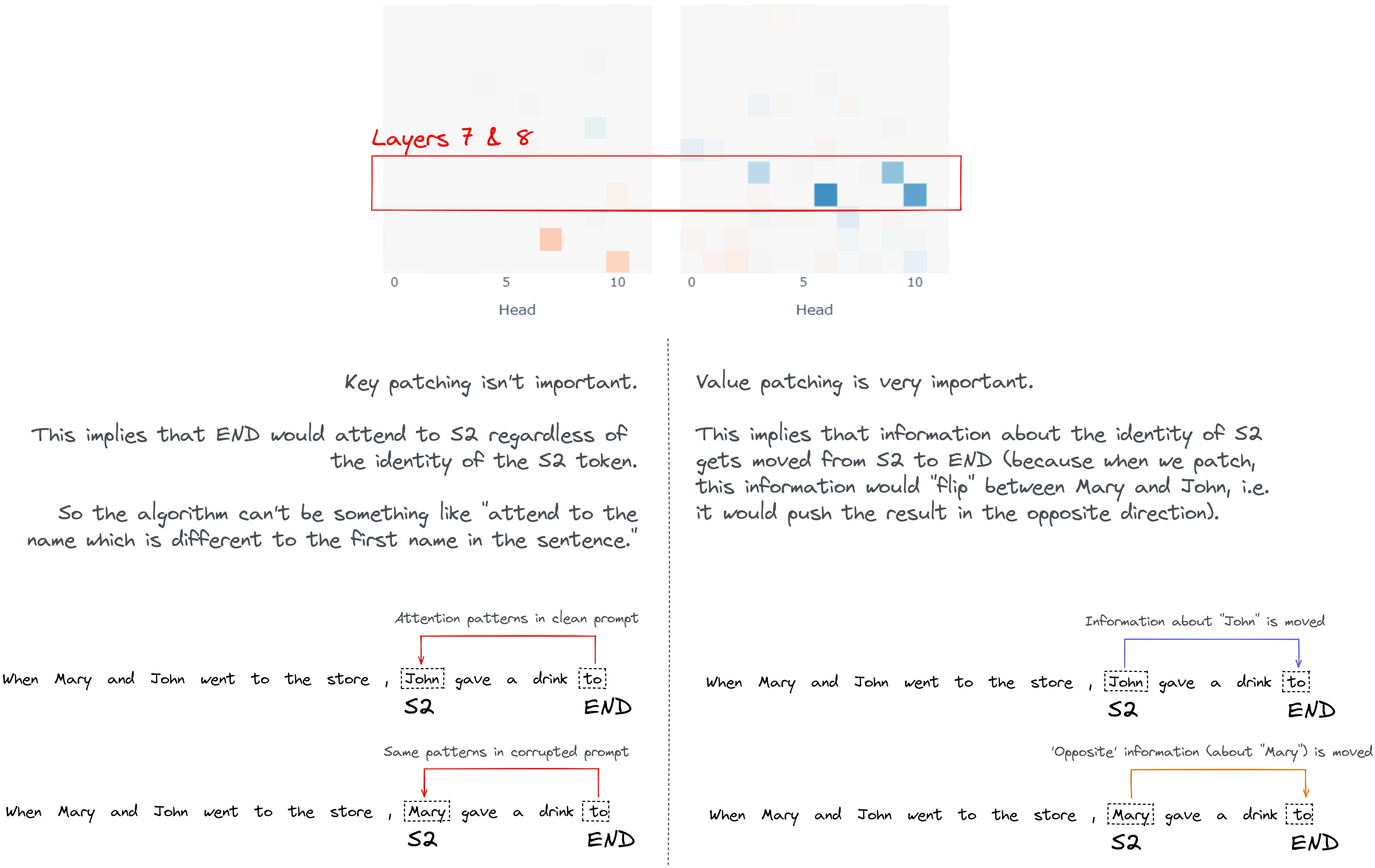
Question - what is the significance of the results for the middle heads (i.e. the important ones in layers 7 & 8)? In particular, how should we interpret the fact that value patching has a much bigger effect than the other two forms of patching?

Hint - if you're confused, try plotting the attention patterns of heads 7.3, 7.9, 8.6, 8.10. You can mostly reuse the code from above when we displayed the output of attention heads.

# Get the heads with largest value patching
# (we know from plot above that these are the 4 heads in layers 7 & 8)
k = 4
top_heads = topk_of_Nd_tensor(act_patch_attn_head_all_pos_every[3], k=k)
# Get all their attention patterns
attn_patterns_for_important_heads: Float[Tensor, "head q k"] = t.stack([
    cache["pattern", layer][:, head].mean(0)
        for layer, head in top_heads
])
# Display results
display(HTML(f"<h2>Top {k} Logit Attribution Heads (from value-patching)</h2>"))
display(cv.attention.attention_patterns(
    attention = attn_patterns_for_important_heads,
    tokens = model.to_str_tokens(tokens[0]),
    attention_head_names = [f"{layer}.{head}" for layer, head in top_heads],
))

Answer

The attention patterns show us that these heads attend from END to S2, so we can guess that they're responsible for moving information from S2 to END which is used to determine the answer. This agrees with our earlier results, when we saw that most of the information gets moved over layers 7 & 8.

The fact that value patching is the most important thing for them suggests that the interesting computation goes into what information they move from S2 to end, rather than why end attends to S2. See the diagram below if you're confused why we can draw this inference.

Consolidating Understanding

OK, let's zoom out and reconsolidate. Here's a recap of the most important observations we have so far:

• Heads 9.9, 9.6, and 10.0 are the most important heads in terms of directly writing to the residual stream. In all these heads, the END attends strongly to the IO.
  • We discovered this by taking the values written by each head in each layer to the residual stream, and projecting them along the logit diff direction by using residual_stack_to_logit_diff. We also looked at attention patterns using circuitsvis.
  • This suggests that these heads are copying IO to end, to use it as the predicted next token.
  • The question then becomes "how do these heads know to attend to this token, and not attend to S?"

• All the action is on S2 until layer 7 and then transitions to END. And that attention layers matter a lot, MLP layers not so much (apart from MLP0, likely as an extended embedding).
  • We discovered this by doing activation patching on resid_pre, attn_out, and mlp_out.
  • This suggests that there is a cluster of heads in layers 7 & 8, which move information from S2 to END. We deduce that this information is how heads 9.9, 9.6 and 10.0 know to attend to IO.
  • The question then becomes "what is this information, how does it end up in the S2 token, and how does END know to attend to it?"

• The significant heads in layers 7 & 8 are 7.3, 7.9, 8.6, 8.10. These heads have high activation patching values for their value vectors, less so for their queries and keys.
  • We discovered this by doing activation patching on the value inputs for these heads.
  • This supports the previous observation, and it tells us that the interesting computation goes into what gets moved from S2 to END, rather than the fact that END attends to S2..
  • We still don't know: "what is this information, and how does it end up in the S2 token?"

• As well as the 2 clusters of heads given above, there's a third cluster of important heads: early heads (e.g. 3.0, 5.5, 6.9) whose query vectors are particularly important for getting good performance.
  • We discovered this by doing activation patching on the query inputs for these heads.

With all this in mind, can you come up with a theory for what these three heads are doing, and come up with a simple model of the whole circuit?

Hint - if you're still stuck, try plotting the attention pattern of head 3.0. The patterns of 5.5 and 6.9 might seem a bit confusing at first (they add complications to the "simplest possible picture" of how the circuit works); we'll discuss them later so they don't get in the way of understanding the core of the circuit.

Answer (and simple diagram of circuit)

If you plotted the attention pattern for head 3.0, you should have seen that S2 paid attention to S1. This suggests that the early heads are detecting when the destination token is a duplicate. So the information that the subject is a duplicate gets stored in S2.

How can the information that the subject token is a duplicate help us predict the token after end? Well, the correct answer (the IO token) is the non-duplicated token. So we can infer that the information that the subject token is a duplicate is used to inhibit the attention of the late heads to the duplicated token, and they instead attend to the non-duplicated token.

To summarise the second half of the circuit: information about this duplicated token is then moved from S2 to end by the middle cluster of heads 7.3, 7.9, 8.6 and 8.10, and this information goes into the queries of the late heads 9.9, 9.6 and 10.0, making them inhibit their attention to the duplicated token. Instead, they attend to IO (copying this token directly to the logits).

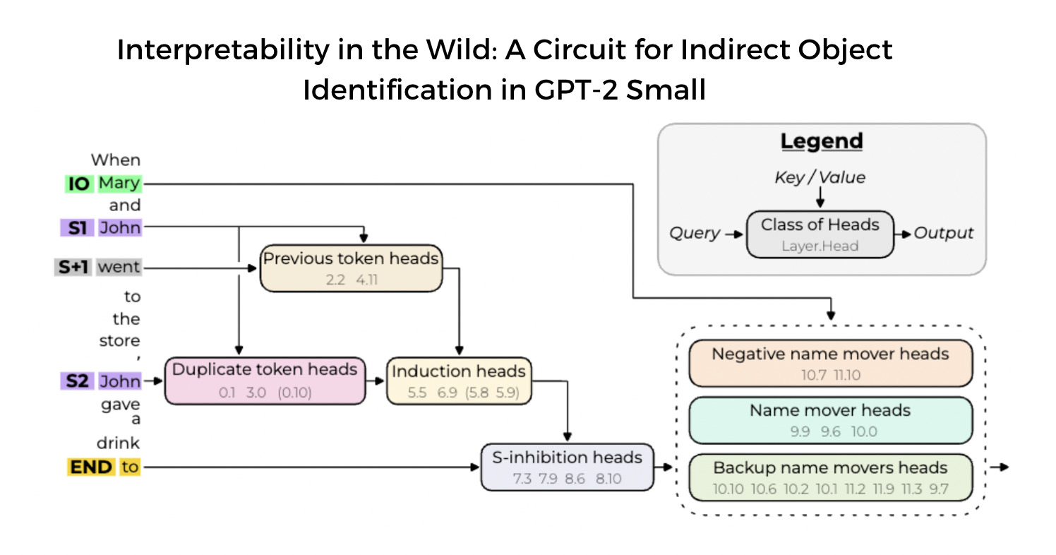
This picture of the circuit turns out to be mostly right. It misses out on some subtleties which we'll discuss shortly, but it's a good rough picture to have in your head. We might illustrate this as follows:

Explanation:

We call the early heads DTH (duplicate token heads), their job is to detect that S2 is a duplicate. The second group of heads are called SIH (S-inhibition heads), their job is to move the duplicated token information from S2 to END. We've illustrated this as them moving the positional information, but in principle this could also be token embedding information (more on this in the final section). * The last group of heads are called NMH (name mover heads), their job is to copy the IO token to the END token, where it is used as the predicted next token (thanks to the S-inihbition heads, these heads don't pay attention to the S token).

Note - if you're still confused about how to interpret this diagram, but you understand induction circuits and how they work, it might help to compare this diagram to one written in the same style which I made for [induction circuits](https://raw.githubusercontent.com/info-arena/ARENA_img/main/misc/ih-simple.png). Also, if you've read my induction heads [LessWrong post](https://www.lesswrong.com/posts/TvrfY4c9eaGLeyDkE/induction-heads-illustrated) and you're confused about how this style of diagram is different from that one, [here](https://raw.githubusercontent.com/info-arena/ARENA_img/main/misc/ih-compared.png) is an image comparing the two diagrams (for induction heads) and explaining how they differ.

Now, let's flesh out this picture a bit more by comparing our results to the paper results. Below is a more complicated version of the diagram in the dropdown above, which also labels the important heads. The diagram is based on the paper's original diagram. Don't worry if you don't understand everything in this diagram; the boundaries of the circuit are fuzzy and the "role" of every head is in this circuit is a leaky abstraction. Rather, this diagram is meant to point your intuitions in the right direction for better understanding this circuit.

Diagram of large circuit

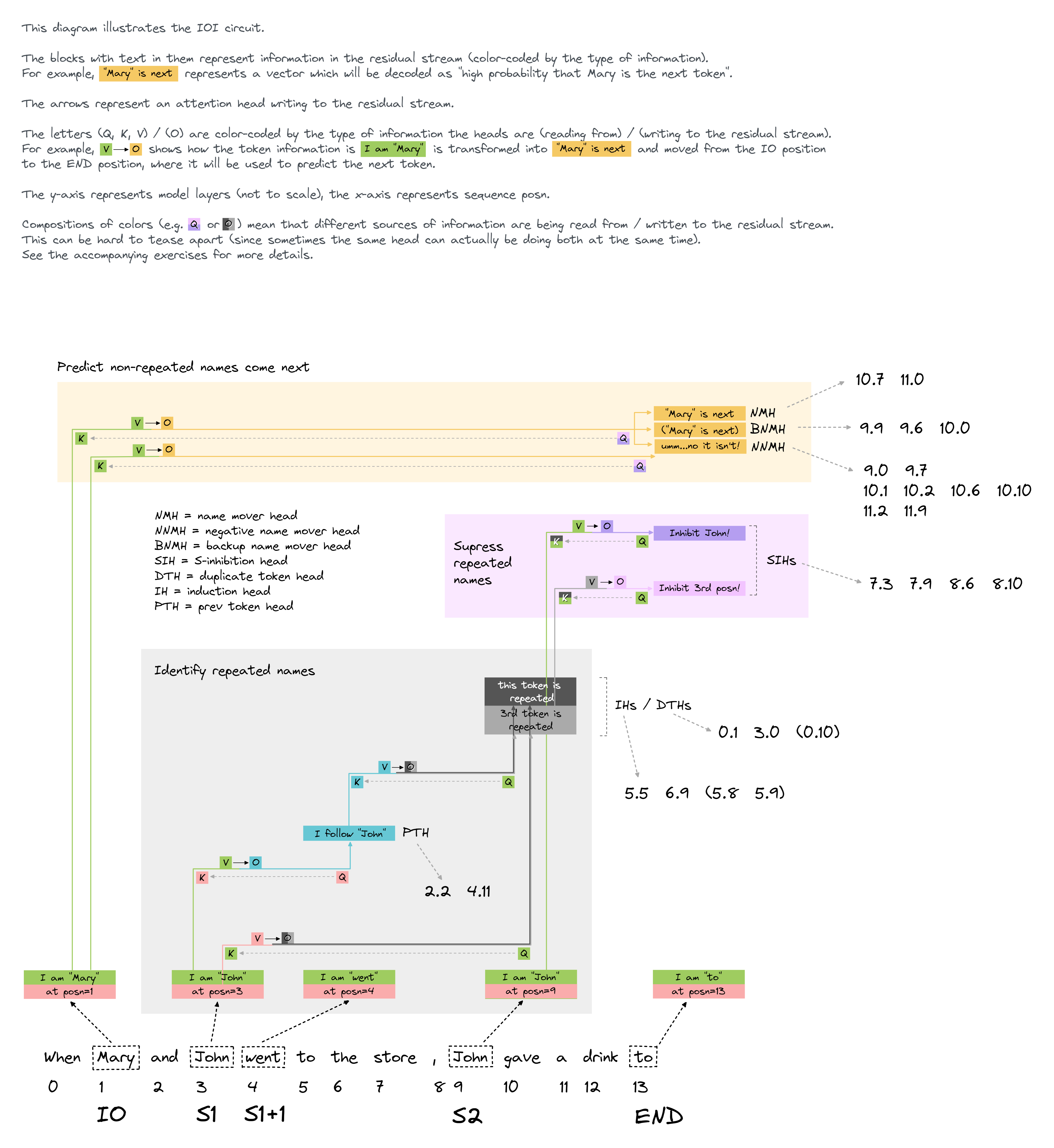
Here are the main ways it differs from the one above:

Induction heads

Rather than just having duplicate token heads in the first cluster of heads, we have two other types of heads as well: previous token heads and induction heads. The induction heads do the same thing as the duplicate token heads, via an induction mechanism. They cause token S2 to attend to S1+1 (mediated by the previous token heads), and their output is used as both a pointer to S1 and as a signal that S1 is duplicated (more on the distinction between these two in the paragraph "Position vs token information being moved" below).

(Note - the original paper's diagram implies the induction heads and duplicate token heads compose with each other. This is misleading, and is not the case.)

Why are induction heads used in this circuit? We'll dig into this more in the bonus section, but one likely possibility is that induction heads are just a thing that forms very early on in training by default, and so it makes sense for the model to repurpose this already-existing machinery for this job. See this paper for more on induction heads, and how / why they form.

Negative & Backup name mover heads

Earlier, we saw that some heads in later layers were actually harming performance. These heads turn out to be doing something pretty similar to name mover heads, but in reverse (i.e. they inhibit the correct answer). It's not obvious why the model does this; the paper speculates that these heads might help the model "hedge" so as to avoid high cross-entropy loss when making mistakes.

Backup name mover heads are possibly even weirder. It turns out that when we ablate the name mover heads, these ones pick up the slack and do the task anyway (even though they don't seem to do it when the NMHs aren't ablated). This is an example of built-in redundancy in the model. One possible explanation is that this resulted from the model being trained with dropout, although this explanation isn't fully satisfying (models trained without dropout still seem to have BNMHs, although they aren't as strong as they are in this model). Like with induction heads, we'll dig into this more in the final section.

Positional vs token information

There are 2 kinds of S-inhibition heads shown in the diagram - ones that inhibit based on positional information (pink), and ones that inhibit based on token information (purple). It's not clear which heads are doing which (and in fact some heads might be doing both!).

The paper has an ingenious way of teasing apart which type of information is being used by which of the S-inhibition heads, which we'll discuss in the final section.

K-composition in S-inhibition heads

When we did activation patching on the keys and values of S-inhibition heads, we found that the values were important and the keys weren't. We concluded that K-composition isn't really happening in these heads, and END must be paying attention to S2 for reasons other than the duplicate token information (e.g. it might just be paying attention to the closest name, or to any names which aren't separated from it by a comma). Although this is mostly true, it turns out that there is a bit of K-composition happening in these heads. We can think of this as the duplicate token heads writing the "duplicated" flag to the residual stream (without containing any information about the identity and position of this token), and this flag is being used by the keys of the S-inhibition heads (i.e. they make END pay attention to S2). In the diagram, this is represented by the dark grey boxes (rather than just the light grey boxes we had in the simplified version). We haven't seen any evidence for this happening yet, but we will in the next section (when we look at path patching).

Note - whether the early heads are writing positional information or "duplicate flag" information to the residual stream is not necessarily related to whether the head is an induction head or a duplicate token head. In principle, either type of head could write either type of information.