3️⃣ Training & Evaluating SAEs

Learning Objectives

• Learn how to train SAEs using SAELens
• Understand how to interpret different metrics during training, and understand when & why SAE training fails to produce interpretable latents
• Get hands-on experience training SAEs in a variety of context: MLP output of TinyStories-1L, residual stream of Gemma-2-2B, attention output of a 2L model, etc
• Understand how to evaluate SAEs, and why simple metrics can be deceptive (not implemented yet)

Introduction

Training SAEs can be very challenging, and new insights are being rapidly discovered. From Joseph Bloom:

SAEs are an unsupervised method which attempts to trade off reconstruction accuracy against interpretability, which we achieve by inducing activation sparsity. Since we don’t have good metrics for interpretability / reconstruction quality, it’s hard to know when we are actually optimizing what we care about. On top of this, we’re trying to pick a good point on the pareto frontier between interpretability and reconstruction quality which is a hard thing to assess well. The main objective is to have your SAE learn a population of sparse latents (which are likely to be interpretable) without having some dense latents (latents which activate all the time and are likely uninterpretable) or too many dead latents (latents which never fire).

In order to help us train SAEs, we've developed a large number of metrics which can be logged while we're training - we'll be discussing more of these later. Many of these metrics are also relevant when performing SAE evaluations - in other words, not trying to measure performance improvements during training, but trying to measure the performance of SAEs post-training in order to assess the beneficial impact of new SAE architectures or training techniques. However, we should be conscious of the fact that different considerations go into metrics for post-training evals vs metrics during training - in particular that post-training metrics only need to be computed once, but it's more important that they tell us a clear and detailed story. For example, techniques like autointerp scoring are promising measures of SAE interpretability, but in their current form are too costly to be performed during training.

Important note before we move on - it's important to draw a distinction between level 1 thinking and level 2 thinking. In this context, level 1 thinking is about interpreting metrics at face value and trying to find training setups which lead to optimal tradeoffs / positions on the Pareto frontier. Level 2 is about asking whether these proxy objectives actually correspond to getting us the SAEs we want, or whether they'll come apart from each other in undesireable ways. For example, feature absorption is one potential issue in SAEs, which casts doubt on the effectiveness of the sparsity penalty. However, these topics are mostly explored in chapter 3 of this material (where we take deep dives into topics like latent absorption, autointerp, latent splitting, etc) as well as the second half of this chapter (where we discuss evals post-training, rather than evals during training). In the first half of this chapter, most of the time you should be thinking at level 1.

Training with SAELens

Like with so many things, SAELens makes training your SAEs relatively straightforward. The code for training is essentially:

from sae_lens import LanguageModelSAERunnerConfig, SAETrainingRunner

runner_cfg = LanguageModelSAERunnerConfig(...)
runner = SAETrainingRunner(runner_cfg)
sae = runner.run()

Training config

The LanguageModelSAERunnerConfig class contains all the parameters necessary to specify how your SAE gets trained. This includes many of the parameters that went into the SAE config (in fact, this class contains a method get_base_sae_cfg_dict() which returns a dictionary that can be used to create the associated SAEConfig object). However, it also includes many other arguments which are specific to the training process itself. You can see the full set of config parameters in the source code for LanguageModelSAERunnerConfig, however for our purposes we can group them into ~7 main categories:

1. Data generation - everything to do with how the data we use to train the SAE is generated & batched. Recall that your SAEs are trained on the activations of a base TransformerLens model, so this includes things like the model name (which should point to a model supported by TransformerLens), hook point in the model, dataset path (which should reference a HuggingFace dataset), etc. We've also included d_in in this category since it's uniquely determined by the hook point you're training on.
2. SAE architecture - everything to do with the SAE architecture, which isn't implied by the data generation parameters. This includes things like d_sae (which you are allowed to use, although in practice we often specify expansion_factor and then d_sae is defined as d_in * expansion_factor), which activation function to use, how our weights are initialized, whether we subtract the decoder bias b_dec from the input, etc.
3. Activations store - everything to do with how the activations are stored and processed during training. Recall we used the ActivationsStore class earlier when we were generating the latent dashboards for our model. During training we also use an instance of this class to store and process batches of activations to feed into our SAE. We need to specify things like how many batches we want to store, how many prompts we want to process at once, etc.
4. Training hyperparameters (standard) - these are the standard kinds of parameters you'd expect to see in an other ML training loop: learning rate & learning rate scheduling, betas for Adam optimizer, etc.
5. Training hyperparameters (SAE-specific) - these are all the parameters which are specific to your SAE training. This means various coefficients like the $L_1$ penalty (as well as warmups for these coefficients), as well as things like the resampling protocol - more on this later. Certain other architectures (e.g. gated) might also come with additional parameters that need specifying.
6. Logging / evals - these control how frequently we log data to Weights & Biases, as well as how often we perform evaluations on our SAE (more on evals in the second half of this exercise set!). Remember that when we talk about evals during training, we're often talking about different kinds of evals than we perform post-training to compare different SAEs to each other (although there's certainly a lot of overlap).
7. Misc - this is a catchall for anything else you might want to specify, e.g. how often you save your model checkpoints, random seeds, device & dtype, etc.

Logging, checkpointing & saving SAEs

For any real training run, you should be logging to Weights and Biases (WandB). This will allow you to track your training progress and compare different runs. To enable WandB, set log_to_wandb=True. The wandb_project parameter in the config controls the project name in WandB. You can also control the logging frequency with wandb_log_frequency and eval_every_n_wandb_logs. A number of helpful metrics are logged to WandB, including the sparsity of the SAE, the mean squared error (MSE) of the SAE, dead latents, and explained variance. These metrics can be used to monitor the training progress and adjust the training parameters. We'll discuss these metrics more in later sections.

Checkpoints allow you to save a snapshot of the SAE and sparsitity statistics during training. To enable checkpointing, set n_checkpoints to a value larger than 0. If WandB logging is enabled, checkpoints will be uploaded as WandB artifacts. To save checkpoints locally, the checkpoint_path parameter can be set to a local directory.

Once you have a set of SAEs that you're happy with, your next step is to share them with the world! SAELens has a upload_saes_to_huggingface() function which makes this easy to do. You'll need to upload a dictionary where the keys are SAE ids, and the values are either SAE objects or paths to an SAE that's been saved using the sae.save_model() method (you can use a combination of both in your dictionary). Note that you'll need to be logged in to your huggingface account either by running huggingface-cli login in the terminal or by setting the HF_TOKEN environment variable to your API token (which should have write access to your repo).

from sae_lens import SAE, upload_saes_to_huggingface

# Create a dictionary of SAEs (keys = SAE ids (can be hook points but don't have to be), values = SAEs)
saes_dict = {
    "blocks.0.hook_resid_pre": layer_0_sae,
    "blocks.1.hook_resid_pre": layer_1_sae,
}

# Upload SAEs to HuggingFace, in your chosen repo (if it doesn't exist, running this code will create it for you)
upload_saes_to_huggingface(
    saes_dict,
    hf_repo_id="your-username/your-sae-repo",
)

# Load all the SAEs back in
uploaded_saes = {
    layer: SAE.from_pretrained(
        release="your-username/your-sae-repo",
        sae_id=f"blocks.{layer}.hook_resid_pre",
        device=str(device)
    )[0]
    for layer in [0, 1]
}

Training advice

In this section we discuss some general training advice, loosely sorted into different sections. Note that much of the advice in this section can carry across different SAE models. However, every different architecture will come with its own set of specific considerations, and it's important to understand what those are when you're training your SAEs.

Metrics

Reconstruction vs sparsity metrics

As we've discussed, most metrics you log to WandB are attempts to measure either reconstruction loss or sparsity, in various different ways. The goal is to monitor how these two different objectives are being balanced, and hopefully find pareto-improvements for them! For reconstruction loss, you want to pay particular attention to MSE loss, CE loss recovered and explained variance. For sparsity, you want to look at the L0 and L1 statistics, as well as the activations histogram (more on that below, since it's more nuanced than "brr line go up/down"!).

The L1 coefficient is the primary lever you have for managing the tradeoff between accurate reconstruction and sparsity. Too high and you get lots of dead latents (although this is mediated by L1 warmup if using a scheduler - see below), too low and your latents will be dense and polysemantic rather than sparse and interpretable.

Another really important point when considering the tradeoff between these two metrics - it might be tempting to use a very high L1 coefficient to get nice sparse interpretable latents, but if this comes at a cost of high reconstruction loss, then there's a real risk that you're not actually learning the model's true behaviour. SAEs are only valuable when they give us a true insight into what the model's representations actually are, and doing interpretability without this risks being just a waste of time. See discussion here between Neel Nanda, Ryan Greenblat & Buck Schlegris for more on this point (note that I don't agree with all the points made in this post, but it raises some highly valuable ideas that SAE researchers would do well to keep in mind).

...but metrics can sometimes be misleading

Although metrics in one of these two groups will often tell a similar story (e.g. explained variance will usually be high when MSE loss is small), they can occasionally detach, and it's important to understand why this might happen. Some examples:

• L0 and L1 both tell you about sparsity, but latent shrinkage makes them detach (it causes smaller L1, not L0)
• MSE loss and KL div / downstream CE both tell you about reconstruction, but they detach because one is myopic and the other is not

As well as being useful to understand these specific examples, it's valuable to put yourself in a skeptical mindset, and understand why these kinds of problems can arise. New metrics are being developed all the time, and some of them might be improvements over current ones while others might carry entirely new and unforseen pitfalls!

Dead latents, resampling & ghost gradients

Dead latents are ones that never fire on any input. These can be a big problem during training, because they don't receive any gradients and so represent permanently lost capacity in your SAE. Two ways of dealing with dead latents, which Anthropic have described in various papers and update posts:

1. Ghost gradients - this describes the method of adding an additional term to the loss, which essentially gives dead latents a gradient signal that pushes them in the direction of explaining more of the autoencoder's residual. Full technical details here.
2. Resampling - at various timesteps we take all our dead latents and randomly re-initialize them to values which help explain more of the residual (specifically, we will randomly select inputs which the SAE fails to reconstruct, and then set dead featurs to be the SAE hidden states corresponding to those inputs).

These techniques are both useful, however they've been reassessed in the time after they were initially introduced, and are now not seen to be as critical as they once were (especially ghost grads). Instead, we use more standard techniques to avoid dead latents, specifically a combination of an appropriately small learning rate and an L1 warmup. We generally recommend people use resampling and not ghost gradients, but to take enough care with your LR and L1 warmup to avoid having to rely on resampling.

Assuming we're not using ghost gradients, resampling is controlled by the following 3 parameters:

• feature_sampling_window, which is how often we resample neurons
• dead_feature_window, which is the size of the window over which we count dead latents each time we resample. This should be smaller than feature_sampling_window
• dead_feature_threshold, which is the threshold below which we consider a latent to be dead & resample it

Dense latents & learning rates

Dense latents are the opposite problem to dead latents: if your learning rate is too small or L1 penalty too small, you'll fail to train latents to the point of being sparse. A dense latent is one that fires too frequently (e.g. on >1/100 or even >1/10 tokens). These latents seem generally uninterpretable, but can help with youre reconstruction loss immensely - essentially it's a way for the SAEs to smuggle not-particularly-sparse possibly-nonlinear computation into your SAE.

It can be difficult to balance dense and dead latents during training. Generally you want to drop your learning rate as far down as it will go, without causing your latents to be dense and your training to be super slow.

Note - what (if any) the right number of dense or dead latents should be in any situation is very much an open question, and depends on your beliefs about the underlying latent distribution in question. One way we can investigate this question is to try and train SAEs in a simpler domain, where the underlying latents are easier to guess about (e.g. OthelloGPT, or TinyStories - both of which we'll discuss later in this chapter).

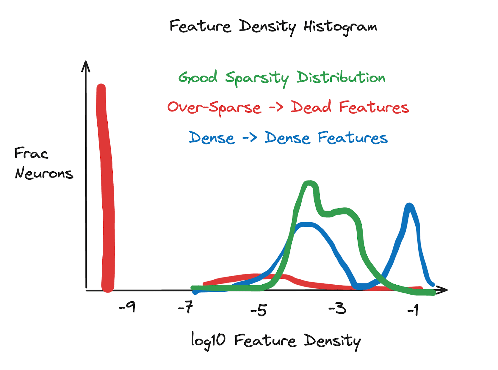
Interpreting the latent density histogram

This section is quoted directly from Joseph Bloom's excellent post on training SAEs:

Latent density histograms are a good measure of SAE quality. We plot the log10 latent sparsity (how often it fires) for all latents. In order to make this easier to operationalize, I’ve drawn a diagram that captures my sense of the issues these histograms help you diagnose. Latent density histograms can be broken down into: - Too Dense: dense latents will occur at a frequency > 1 / 100. Some dense-ish latents are likely fine (such as a latent representing that a token begins with a space) but too many is likely an issue. - Too Sparse: Dead latents won’t be sampled so will turn up at log10(epsilon), for epsilon added to avoid logging 0 numbers. Too many of these mean you’re over penalizing with L1. - Just-Right: Without too many dead or dense latents, we see a distribution that has most mass between -5 or -4 and -3 log10 latent sparsity. The exact range can vary depending on the model / SAE size but the dense or dead latents tend to stick out.

Architecture

Width

Wider SAEs (i.e. ones with a larger expansion factor / larger d_sae) will take longer to train, but will often have better performance on metrics like explained variance. As we mention in the previous section on metrics, it's important not to over-interpret an SAE which doesn't explain the majority of the model's true performance, because at that point we're learning things about our SAE but not about our model!

It's also good to be aware of concepts like feature splitting when choosing width. You might still get interpretable latents for a variety of different widths, even if those latents are often related to each other via some kind of feature splitting. Feature absorption is a different (possibly more severe) kind of problem, which might happen more with wider SAEs but could in theory happen at any width.

Gated models

We've discussed gated models in previous sections, in comparison to other architectures like standard or topk. In most cases, we recommend picking gated models in your training because currently they seem to outperform other simple architectures (not counting significant paradigm-shifting SAE-like architectures such as transcoders). From Neel Nanda:

"I ... think [the DeepMind Gated SAEs paper] is worth reading as a good exemplar of how to rigorously evaluate whether an SAE change was an improvement."

If you're not using gated models, we at least recommend something like topk, since they do offer some similar benefits to Gated models (e.g. addressing the shrinkage issue).

Performance Optimization

Datasets & streaming

cfg = LanguageModelSAERunnerConfig(
    dataset_path="apollo-research/roneneldan-TinyStories-tokenizer-gpt2",
    is_dataset_tokenized=True,
    prepend_bos=True,
    streaming=True,
    train_batch_size_tokens=4096,
    context_size=512,
)

The is_dataset_tokenized argument should be True if the dataset is pre-tokenized, False if the dataset is not tokenized. A pre-tokenized dataset is one that has already been tokenized & batched for all subsequent training runs. This will speed up SAE training, because you don't need to tokenize the dataset on the fly. See this tutorial for information on how to pre-tokenize your own dataset, if the one you're working with isn't pre-tokenized. However for now we don't need to worry about that, because ours is pre-tokenized. You can find a non-exhaustive list of pre-tokenized datasets here.

Regardless of tokenization, the datasets SAELens works with are often very large, and take a lot of time & disk space to download from HuggingFace. To speed this up, you can set streaming=True in the config. This will stream the dataset from Huggingface during training, which will allow training to start immediately and save disk space.

Context size

The context_size parameter controls the length of the prompts fed to the model. Larger context sizes will result in better SAE performance, but will also slow down training. Each training batch will be tokens of size train_batch_size_tokens * context_size.

Misc. tips

• We recommend sticking to the default beta values of (0.9, 0.999), in line with Anthropic's update.
• How long should you be training for? The generic ML advice applies here - when you stop seeing improvements in your loss curves, then it's probably time to stop training! You can also use other successful runs as a reference, e.g. the ones described in this post. The linked training runs here are also likely good.
• Training data should match what the model was trained on. For IT models / SAEs chat data would be good but hard to find, DM uses Open Web Text.

The rest of this chapter (before evals) is split into three sections:

1. We present an example training run, where an SAE is trained on the output of the final MLP layer of a TinyStories-1L model. This will be an opportunity to actually see what a start-to-finish training run looks like, and also have a look at some example metrics on the WandB page.
2. As an exercise, we present a series of different training runs on this same model, each of which have something wrong with them. Your task will be to try and use the various metrics to diagnose what's going wrong with these runs, as well as finding the trainer config settings that might have been responsible.
3. Lastly, we'll present a series of case studies which showcase various different instances of SAE training. They'll use a variety of different base models (from 1L models to Gemma-2B), different hook points (from residual stream to MLP output to attention output), and different SAE architectures (gated, transcoder, etc). For each of these, we'll provide some tips on training, and how we recommend you approach them differently based on the specifics of what it is you're training. We will also provide sample code if you feel stuck, although this sample code may well be suboptimal and we leave it to you to find something even better!

# We start by emptying memory of all large tensors & objects (since we'll be loading in a lot of different models in the coming sections)
THRESHOLD = 0.1  # GB
for obj in gc.get_objects():
    try:
        if isinstance(obj, t.nn.Module) and utils.get_tensors_size(obj) / 1024**3 > THRESHOLD:
            if hasattr(obj, "cuda"):
                obj.cpu()
            if hasattr(obj, "reset"):
                obj.reset()
    except:
        pass

Training Case Study: TinyStories-1L, MLP-out

In our first training case study, we'll train an SAE on the output of the final (only) MLP layer of a TinyStories model. TinyStories is a synthetic dataset consisting of short stories, which contains a vocabulary of ~1500 words (mostly just common words that typical 3-4 year old children can understand). Each story is also relatively short, self-contained, and contains a basic sequence of events which can often be causally inferred from the previous context. Example sequences look like:

Once upon a time, there was a little girl named Lily. Lily liked to pretend she was a popular princess. She lived in a big castle with her best friends, a cat and a dog. One day, while playing in the castle, Lily found a big cobweb. The cobweb was in the way of her fun game. She wanted to get rid of it, but she was scared of the spider that lived there. Lily asked her friends, the cat and the dog, to help her. They all worked together to clean the cobweb. The spider was sad, but it found a new home outside. Lily, the cat, and the dog were happy they could play without the cobweb in the way. And they all lived happily ever after.

This dataset gives us a useful playground for interpretability analysis, because the kinds of features which it is useful for models to learn in order to minimize predictive loss on this dataset are far narrower and simpler than they would be for models trained on more complex natural language datasets.

Let's load in the model we'll be training our SAE on, and get a sense for how models trained on this dataset behave by generating text from it. This is a useful first step when it comes to thinking about what features the model is likely to have learned.

tinystories_model = HookedSAETransformer.from_pretrained("tiny-stories-1L-21M")

completions = [
    (i, tinystories_model.generate("Once upon a time", temperature=1, max_new_tokens=50))
    for i in range(5)
]

print(tabulate(completions, tablefmt="simple_grid", maxcolwidths=[None, 100]))

┌───┬──────────────────────────────────────────────────────────────────────────────────────────────────────┐
│ 0 │ Once upon a time, there was a little girl called Joy. She was so enthusiastic and loved to explore.  │
│   │ One day, Joy decided to go outside and explored a nearby forest. It was a beautiful summer day, and  │
│   │ the solitude. Joy soon realized it was                                                               │
├───┼──────────────────────────────────────────────────────────────────────────────────────────────────────┤
│ 1 │ Once upon a time, a gifted little girl was very happy. Every day she would paint and hang books on   │
│   │ the wall. She painted pictures, ribbons and flowers. The wall was so happy with the result. One day, │
│   │ something horrible happened. It started                                                              │
├───┼──────────────────────────────────────────────────────────────────────────────────────────────────────┤
│ 2 │ Once upon a time, there was a brown bug called a jet. It flew very fast and traveled very far. One   │
│   │ day, he came across a big, playful comet flying around so far that went off over mountains.  He came │
│   │ across a stream with swirling water                                                                  │
├───┼──────────────────────────────────────────────────────────────────────────────────────────────────────┤
│ 3 │ Once upon a time, there was a boy named Jack. He was a kind and humble man, and often Julia would    │
│   │ visit the beach.  One day, Jack asked, "What place are we going to do today?"  Julia said, "I        │
├───┼──────────────────────────────────────────────────────────────────────────────────────────────────────┤
│ 4 │ Once upon a time, there was a famous man. He was known as the most famous guy in the sky. Everyone   │
│   │ believed him and started to pay him what he had been doing.  The famous man then saw a 3 year old    │
│   │ child playing in the yard.                                                                           │
└───┴──────────────────────────────────────────────────────────────────────────────────────────────────────┘

We can also spot-check model abilities with utils.test_prompt, from the TransformerLens library:

test_prompt(
    "Once upon a time, there was a little girl named Lily. She lived in a big, happy little girl. On her big adventure,",
    [" Lily", " she", " he"],
    tinystories_model,
)

Tokenized prompt: ['<|endoftext|>', 'Once', ' upon', ' a', ' time', ',', ' there', ' was', ' a', ' little', ' girl', ' named', ' Lily', '.', ' She', ' lived', ' in', ' a', ' big', ',', ' happy', ' little', ' girl', '.', ' On', ' her', ' big', ' adventure', ',']
Tokenized answers: [[' Lily'], [' she'], [' he']]

Performance on answer tokens:
Rank: 1        Logit: 18.81 Prob: 13.46% Token: | Lily|
Rank: 0        Logit: 20.48 Prob: 71.06% Token: | she|
Rank: 104      Logit: 11.23 Prob:  0.01% Token: | he|
Top 0th token. Logit: 20.48 Prob: 71.06% Token: | she|
Top 1th token. Logit: 18.81 Prob: 13.46% Token: | Lily|
Top 2th token. Logit: 17.35 Prob:  3.11% Token: | the|
Top 3th token. Logit: 17.26 Prob:  2.86% Token: | her|
Top 4th token. Logit: 16.74 Prob:  1.70% Token: | there|
Top 5th token. Logit: 16.43 Prob:  1.25% Token: | they|
Top 6th token. Logit: 15.80 Prob:  0.66% Token: | all|
Top 7th token. Logit: 15.64 Prob:  0.56% Token: | things|
Top 8th token. Logit: 15.28 Prob:  0.39% Token: | one|
Top 9th token. Logit: 15.24 Prob:  0.38% Token: | lived|
Ranks of the answer tokens: [[(' Lily', 1), (' she', 0), (' he', 104)]]

In the output above, we see that the model assigns ~ 70% probability to " she" being the next token (with " he" ranked much lower at .01%), and a 13% chance to " Lily" being the next token. Other names like Lucy or Anna are not highly ranked.

For a more detailed view than offered by utils.test_prompt, we can use the circuitsvis library to produce visualizations. In the following code, we visualize logprobs for the next token for all of the tokens in our generated sequence. Darker tokens indicate the model assigning a higher probability to the actual next token, and you can also hover over tokens to see the top 10 predictions by their logprob.

completion = tinystories_model.generate(
    "Once upon a time", temperature=1, verbose=False, max_new_tokens=200
)

cv.logits.token_log_probs(
    tinystories_model.to_tokens(completion),
    tinystories_model(completion).squeeze(0).log_softmax(dim=-1),
    tinystories_model.to_string,
)

Before we start training our model, we recommend you play around with this code. Some things to explore:

• Which tokens does the model assign high probability to? Can you see how the model should know which word comes next?
• Do the rankings of tokens seem sensible to you? What about where the model doesn't assign a high probability to the token which came next?
• Try changing the temperature of the generated completion, to make the model sample more or less likely trajectories. How does this affect the probabilities?

Now we're ready to train out SAE. We'll make a runner config, instantiate the runner and the rest is taken care of for us!

During training, you use weights and biases to check key metrics which indicate how well we are able to optimize the variables we care about. You can reorganize your WandB dashboard to put important metrics like L0, CE loss score, explained variance etc in one section at the top. We also recommend you make a run comparer for your different runs, whenever performing multiple training runs (e.g. hyperparameter sweeps).

If you've disabled gradients, remember to re-enable them using t.set_grad_enabled(True) before training.

total_training_steps = 30_000  # probably we should do more
batch_size = 4096
total_training_tokens = total_training_steps * batch_size

lr_warm_up_steps = l1_warm_up_steps = total_training_steps // 10  # 10% of training
lr_decay_steps = total_training_steps // 5  # 20% of training

cfg = LanguageModelSAERunnerConfig(
    #
    # Data generation
    model_name="tiny-stories-1L-21M",  # our model (more options here: https://neelnanda-io.github.io/TransformerLens/generated/model_properties_table.html)
    hook_name="blocks.0.hook_mlp_out",
    hook_layer=0,
    d_in=tinystories_model.cfg.d_model,
    dataset_path="apollo-research/roneneldan-TinyStories-tokenizer-gpt2",  # tokenized language dataset on HF for the Tiny Stories corpus.
    is_dataset_tokenized=True,
    prepend_bos=True,  # you should use whatever the base model was trained with
    streaming=True,  # we could pre-download the token dataset if it was small.
    train_batch_size_tokens=batch_size,
    context_size=512,  # larger is better but takes longer (for tutorial we'll use a short one)
    #
    # SAE architecture
    architecture="gated",
    expansion_factor=16,
    b_dec_init_method="zeros",
    apply_b_dec_to_input=True,
    normalize_sae_decoder=False,
    scale_sparsity_penalty_by_decoder_norm=True,
    decoder_heuristic_init=True,
    init_encoder_as_decoder_transpose=True,
    #
    # Activations store
    n_batches_in_buffer=64,
    training_tokens=total_training_tokens,
    store_batch_size_prompts=16,
    #
    # Training hyperparameters (standard)
    lr=5e-5,
    adam_beta1=0.9,
    adam_beta2=0.999,
    lr_scheduler_name="constant",  # controls how the LR warmup / decay works
    lr_warm_up_steps=lr_warm_up_steps,  # avoids large number of initial dead features
    lr_decay_steps=lr_decay_steps,  # helps avoid overfitting
    #
    # Training hyperparameters (SAE-specific)
    l1_coefficient=4,
    l1_warm_up_steps=l1_warm_up_steps,
    use_ghost_grads=False,  # we don't use ghost grads anymore
    feature_sampling_window=2000,  # how often we resample dead features
    dead_feature_window=1000,  # size of window to assess whether a feature is dead
    dead_feature_threshold=1e-4,  # threshold for classifying feature as dead, over window
    #
    # Logging / evals
    log_to_wandb=True,  # always use wandb unless you are just testing code.
    wandb_project="arena-demos-tinystories",
    wandb_log_frequency=30,
    eval_every_n_wandb_logs=20,
    #
    # Misc.
    device=str(device),
    seed=42,
    n_checkpoints=5,
    checkpoint_path="checkpoints",
    dtype="float32",
)

print("Comment this code out to train! Otherwise, it will load in the already trained model.")
# t.set_grad_enabled(True)
# runner = SAETrainingRunner(cfg)
# sae = runner.run()

hf_repo_id = "callummcdougall/arena-demos-tinystories"
sae_id = cfg.hook_name

# upload_saes_to_huggingface({sae_id: sae}, hf_repo_id=hf_repo_id)

tinystories_sae = SAE.from_pretrained(release=hf_repo_id, sae_id=sae_id, device=str(device))[0]

Once you've finished training your SAE, you can try using the following code from the sae_vis library to visualize your SAE's latents.

(Note - this code comes from a branch of the sae_vis library, which soon will be merged into main, and will also be more closely integrated with the rest of SAELens. For example, this method currently works by directly taking a batch of tokens, but in the future it will probably take an ActivationsStore object to make things easier.)

First, we get a batch of tokens from the dataset:

dataset = load_dataset(cfg.dataset_path, streaming=True)
batch_size = 1024
tokens = t.tensor(
    [x["input_ids"] for i, x in zip(range(batch_size), dataset["train"])],
    device=str(device),
)
print(tokens.shape)

Next, we create the visualization and save it (you'll need to download the file and open it in a browser to view). Note that if you get OOM errors then you can reduce the number of features visualized, or decrease either the batch size or context length.

sae_vis_data = SaeVisData.create(
    sae=tinystories_sae,
    model=tinystories_model,
    tokens=tokens,
    cfg=SaeVisConfig(features=range(16)),
    verbose=True,
)
sae_vis_data.save_feature_centric_vis(
    filename=str(section_dir / "feature_vis.html"),
    verbose=True,
)

# If this display code doesn't work, you might need to download the file & open in browser to see it
with open(str(section_dir / "feature_vis.html")) as f:
    display(HTML(f.read()))

Exercise - identify good and bad training curves

Here is a link to a WandB project page with seven training runs. The first one (Run #0) is a "good" training run (at least compared to the others), and can be thought of as a baseline. Each of the other 6 runs (labelled Run #1 - Run #6) has some particular issue with it. Your task will be to identify the issue (i.e. from one or more of the metrics plots), and find the root cause of the issue from looking at the configs (you can compare the configs to each other in the "runs" tab). Note that we recommend trying to identify the issue from the plots first, rather than immediately jumping to the config and looking for a diff between it and the good run. You'll get most value out of the exercises by using the following pattern when assessing each run:

1. Looking at the metrics, and finding some which seem like indications of poor SAE quality
2. Based on these metrics, try and guess what might be going wrong in the config
3. Look at the config, and test whether your guess was correct.

Also, a reminder - you can look at a run's density histogram plot, although you can only see this when you're looking at the page for a single run (as opposed to the project page).

Use the dropdowns below to see the answer for each of the runs. Note, the first few are more important to get right, as the last few are more difficult and don't always have obvious root causes.

More case studies

Train on attn output of a 2L model

In this section, we encourage you to try and train a 2-layer attention-only SAE. The name of the TransformerLens model is "attn-only-2l-demo"; you can load it in and inspect it to see what it looks like.

A good target for this section would be to train SAEs on the attention output (i.e. hook_z) for both layers 0 and 1, and see if you can find pairs of features which form induction circuits. You might want to revisit earlier sections for a guide on how to do this (e.g. "finding features" from section 1, or "feature-to-feature gradients" from section 2).

Some tips:

• You might want to experiment with different expansion factors for your attention SAEs, since the appropriate expansion factor will be different depending on the model you're training & hook point you're looking at.
• You'll need a different dataset, which either isn't pretokenized or whose tokenization matches the tokenizer of the model you're training on. You can check the latter with model.cfg.tokenizer_name, and see if any of the pretokenized datasets here support this tokenizer.

We've given you some reasonable default parameters below, to get you started. You can either modify these / perform hyperparameter sweeps using them as a baseline, or if you want to be ambitious then you can try and write a config from scratch, just starting from the config we gave you in the previous section.

attn_model = HookedSAETransformer.from_pretrained("attn-only-2l-demo")

total_training_steps = 30_000  # probably we should do more
batch_size = 4096
total_training_tokens = total_training_steps * batch_size

lr_warm_up_steps = l1_warm_up_steps = total_training_steps // 10  # 10% of training
lr_decay_steps = total_training_steps // 5  # 20% of training

layer = 0

cfg = LanguageModelSAERunnerConfig(
    #
    # Data generation
    model_name="attn-only-2l-demo",
    hook_name=f"blocks.{layer}.attn.hook_z",
    hook_layer=layer,
    d_in=attn_model.cfg.d_head * attn_model.cfg.n_heads,
    dataset_path="apollo-research/Skylion007-openwebtext-tokenizer-EleutherAI-gpt-neox-20b",
    is_dataset_tokenized=True,
    prepend_bos=True,  # you should use whatever the base model was trained with
    streaming=True,  # we could pre-download the token dataset if it was small.
    train_batch_size_tokens=batch_size,
    context_size=attn_model.cfg.n_ctx,
    #
    # SAE architecture
    architecture="gated",
    expansion_factor=16,
    b_dec_init_method="zeros",
    apply_b_dec_to_input=True,
    normalize_sae_decoder=False,
    scale_sparsity_penalty_by_decoder_norm=True,
    decoder_heuristic_init=True,
    init_encoder_as_decoder_transpose=True,
    #
    # Activations store
    n_batches_in_buffer=64,
    training_tokens=total_training_tokens,
    store_batch_size_prompts=16,
    #
    # Training hyperparameters (standard)
    lr=1e-4,
    adam_beta1=0.9,
    adam_beta2=0.999,
    lr_scheduler_name="constant",
    lr_warm_up_steps=lr_warm_up_steps,  # avoids large number of initial dead features
    lr_decay_steps=lr_decay_steps,
    #
    # Training hyperparameters (SAE-specific)
    l1_coefficient=2,
    l1_warm_up_steps=l1_warm_up_steps,
    use_ghost_grads=False,  # we don't use ghost grads anymore
    feature_sampling_window=1000,  # how often we resample dead features
    dead_feature_window=500,  # size of window to assess whether a feature is dead
    dead_feature_threshold=1e-4,  # threshold for classifying feature as dead, over window
    #
    # Logging / evals
    log_to_wandb=True,  # always use wandb unless you are just testing code.
    wandb_project="arena-demos-attn2l",
    wandb_log_frequency=30,
    eval_every_n_wandb_logs=20,
    #
    # Misc.
    device=str(device),
    seed=42,
    n_checkpoints=5,
    checkpoint_path="checkpoints",
    dtype="float32",
)

print("Comment this code out to train! Otherwise, it will load in the already trained model.")
# t.set_grad_enabled(True)
# runner = SAETrainingRunner(cfg)
# sae = runner.run()

hf_repo_id = "callummcdougall/arena-demos-attn2l"
sae_id = f"{cfg.hook_name}-v2"

# upload_saes_to_huggingface({sae_id: sae}, hf_repo_id=hf_repo_id)

attn_sae = SAE.from_pretrained(release=hf_repo_id, sae_id=sae_id, device=str(device))[0]

# Get batch of tokens
dataset = load_dataset(cfg.dataset_path, streaming=True)
batch_size = 1024
seq_len = 256
tokens = t.tensor(
    [x["input_ids"][: seq_len - 1] for i, x in zip(range(batch_size), dataset["train"])],
    device=str(device),
)
bos_token = t.tensor([attn_model.tokenizer.bos_token_id for _ in range(batch_size)], device=device)
tokens = t.cat([bos_token.unsqueeze(1), tokens], dim=1)
assert tokens.shape == (batch_size, seq_len)

# Get a subset of live latents (probably not getting all of them, with only 100 seqs)
acts_post_hook_name = f"{attn_sae.cfg.hook_name}.hook_sae_acts_post"
_, cache = attn_model.run_with_cache_with_saes(
    tokens[:100], saes=[attn_sae], names_filter=acts_post_hook_name
)
acts = cache[acts_post_hook_name]
alive_feats = (acts.flatten(0, 1) > 1e-8).any(dim=0).nonzero().squeeze().tolist()
print(f"Alive latents: {len(alive_feats)}/{attn_sae.cfg.d_sae}\n")
del cache

# Create vis from live latents
sae_vis_data = SaeVisData.create(
    sae=attn_sae,
    model=attn_model,
    tokens=tokens,
    cfg=SaeVisConfig(features=alive_feats[:32]),
    verbose=True,
    clear_memory_between_batches=True,
)
sae_vis_data.save_feature_centric_vis(filename=str(section_dir / "sae_vis_attn.html"))

# If this display code doesn't work, you might need to download the file & open in browser to see it
with open(str(section_dir / "sae_vis_attn.html")) as f:
    display(HTML(f.read()))

Train on Gemma-2B residual stream

In this section, you should try and train on the residual stream of gemma-2-2b. You can jump back to the section on GemmaScope (immediately before feature steering) to both review what the Gemma model series is, and also get a sense of the GemmaScope architecture (which should help guide your own architectural choices). Reminder that you can find a list of suitable pretokenized datasets for various different models here.

We've included an example config below containing some reasonable default parameters, which you can use to get started.

Note that you might find training on gemma-2-2b very compute and memory-intensive, and for that reason you might want to work on some of the other training exercises in this section before moving onto Gemma. Even with access to an A100 (e.g. Colab Pro+), training to the point of quality learned features can be on the order of days, not hours.

total_training_steps = 300_000  # Calculated from training_tokens / batch_size
batch_size = 4096
total_training_tokens = total_training_steps * batch_size

lr_warm_up_steps = l1_warm_up_steps = total_training_steps // 10  # 10% of training
lr_decay_steps = total_training_steps // 5  # 20% of training

layer = 12

cfg = LanguageModelSAERunnerConfig(
    #
    # Data generation
    model_name="gemma-2-2b",
    hook_name=f"blocks.{layer}.hook_resid_post",
    hook_layer=layer,
    d_in=2304,
    dataset_path="chanind/openwebtext-gemma",
    is_dataset_tokenized=True,
    # dataset_path="HuggingFaceFW/fineweb",
    # is_dataset_tokenized=False,
    prepend_bos=True,
    streaming=True,
    train_batch_size_tokens=batch_size,
    context_size=1024,
    #
    # SAE architecture
    architecture="gated",
    expansion_factor=8,
    b_dec_init_method="zeros",
    apply_b_dec_to_input=True,
    normalize_sae_decoder=False,
    scale_sparsity_penalty_by_decoder_norm=True,
    decoder_heuristic_init=True,
    init_encoder_as_decoder_transpose=True,
    #
    # Activations store
    n_batches_in_buffer=16,
    training_tokens=total_training_tokens,
    store_batch_size_prompts=8,
    #
    # Training hyperparameters (standard)
    lr=5e-5,
    adam_beta1=0.9,
    adam_beta2=0.999,
    lr_scheduler_name="constant",
    lr_warm_up_steps=lr_warm_up_steps,
    lr_decay_steps=lr_decay_steps,
    #
    # Training hyperparameters (SAE-specific)
    l1_coefficient=2,
    l1_warm_up_steps=l1_warm_up_steps,
    use_ghost_grads=False,
    feature_sampling_window=5000,
    dead_feature_window=5000,
    dead_feature_threshold=1e-6,
    #
    # Logging / evals
    log_to_wandb=True,
    wandb_project="arena-demos-gemma2b",
    wandb_log_frequency=50,
    eval_every_n_wandb_logs=20,
    #
    # Misc.
    device=str(device),
    seed=42,
    n_checkpoints=5,
    checkpoint_path="checkpoints",
    dtype="float32",
)


print("This model hasn't been trained yet!")
# t.set_grad_enabled(True)
# runner = SAETrainingRunner(cfg)
# sae = runner.run()

# hf_repo_id = "callummcdougall/arena-demos-gemma2b"
# sae_id = cfg.hook_name

# upload_saes_to_huggingface({sae_id: sae}, hf_repo_id=hf_repo_id)

# gemma_sae = SAE.from_pretrained(
#     release=hf_repo_id, sae_id=sae_id, device=str(device)
# )[0]

Train on OthelloGPT

OthelloGPT is a model that was trained to predict legal moves in Othello. It's an interesting domain for studying SAEs, because it's simpler than most natural language datasets, but it's also more complex than the vast majority of toy problems (because to track which squares are legal, you have to keep track of a large number of possible captures and recaptures). Furthermore, research by Neel Nanda strongly suggests that OthelloGPT contains a linear board state model, which means:

• We might expect SAEs trained on the residual stream to be able to extract these board state representations,
• We might expect SAEs trained on MLP layers or attention outputs to capture some computation that is performed on / used to create these linear representations.

Training & exploring SAEs on OthelloGPT would make a really exciting project, since it serves as a good testbed for applying lots of new techniques in SAE interpretability (including many of the ones we've discussed earlier in these exercises). We've included some sample code to train a model below; again it's probably quite under-optimized and you're invited to try various methods of improving it (or trying it on different layers / different parts of the base model).

model_name = "othello-gpt"
othellogpt = HookedSAETransformer.from_pretrained(model_name)

layer = 5
training_tokens = int(1e8)
train_batch_size_tokens = 2048
n_steps = int(training_tokens / train_batch_size_tokens)

cfg = LanguageModelSAERunnerConfig(
    #
    # Data generation
    model_name=model_name,
    hook_name=f"blocks.{layer}.mlp.hook_post",
    hook_layer=layer,
    d_in=othellogpt.cfg.d_mlp,
    dataset_path="taufeeque/othellogpt",
    is_dataset_tokenized=True,
    prepend_bos=False,
    streaming=True,
    train_batch_size_tokens=train_batch_size_tokens,
    context_size=othellogpt.cfg.n_ctx,  # = 59, we only train on tokens up to (not including) the last one
    seqpos_slice=(5, -5),  # we don't train on the first or last 5 sequence positions
    #
    # SAE achitecture
    architecture="gated",
    expansion_factor=8,
    b_dec_init_method="zeros",
    apply_b_dec_to_input=True,
    normalize_sae_decoder=False,
    scale_sparsity_penalty_by_decoder_norm=True,
    decoder_heuristic_init=True,
    init_encoder_as_decoder_transpose=True,
    #
    # Activations store
    n_batches_in_buffer=32,
    store_batch_size_prompts=16,
    training_tokens=training_tokens,
    #
    # Training hyperparameters (standard)
    lr=2e-4,
    adam_beta1=0.9,
    adam_beta2=0.999,
    lr_scheduler_name="constant",
    lr_warm_up_steps=int(0.2 * n_steps),
    lr_decay_steps=int(0.2 * n_steps),
    #
    # Training hyperparameters (SAE-specific)
    l1_coefficient=5,
    l1_warm_up_steps=int(0.2 * n_steps),
    use_ghost_grads=False,
    feature_sampling_window=1000,
    dead_feature_window=500,
    dead_feature_threshold=1e-5,
    #
    # Logging / evals
    log_to_wandb=True,
    wandb_project="othello_gpt_sae_16_09",
    wandb_log_frequency=30,
    eval_every_n_wandb_logs=10,
    #
    # Misc.
    device=str(device),
    seed=42,
    n_checkpoints=5,
    checkpoint_path="checkpoints",
    dtype="float32",
)

# t.set_grad_enabled(True)
# runner = SAETrainingRunner(cfg, override_dataset=override_dataset)
# sae = runner.run()

hf_repo_id = "callummcdougall/arena-demos-othellogpt"
sae_id = f"{cfg.hook_name}-v1"

# upload_saes_to_huggingface({sae_id: sae}, hf_repo_id=hf_repo_id)

othellogpt_sae = SAE.from_pretrained(release=hf_repo_id, sae_id=sae_id, device=str(device))[0]

Now, creating a visualization for this SAE:

def hf_othello_load(filename):
    path = hf_hub_download(repo_id=hf_repo_id, filename=filename)
    return t.load(path, weights_only=True, map_location=device)


def load_othello_vocab():
    all_squares = [r + c for r in "ABCDEFGH" for c in "01234567"]
    legal_squares = [sq for sq in all_squares if sq not in ["D3", "D4", "E3", "E4"]]
    # Model's vocabulary = all legal squares (plus "pass")
    vocab_dict = {
        token_id: str_token for token_id, str_token in enumerate(["pass"] + legal_squares)
    }
    # Probe vocabulary = all squares on the board
    vocab_dict_probes = {token_id: str_token for token_id, str_token in enumerate(all_squares)}
    return {
        "embed": vocab_dict,
        "unembed": vocab_dict,
        "probes": vocab_dict_probes,
    }


othello_tokens = hf_othello_load("tokens.pt")
othello_target_logits = hf_othello_load("target_logits.pt")
othello_linear_probes = hf_othello_load("linear_probes.pt")
print(f"{othello_tokens.shape=}")

# Get live features
acts_post_hook_name = f"{othellogpt_sae.cfg.hook_name}.hook_sae_acts_post"
_, cache = othellogpt.run_with_cache_with_saes(
    othello_tokens[:500], saes=[othellogpt_sae], names_filter=acts_post_hook_name
)
acts = cache[acts_post_hook_name]
alive_feats = (acts[:, 5:-5].flatten(0, 1) > 1e-8).any(dim=0).nonzero().squeeze().tolist()
print(f"Alive features: {len(alive_feats)}/{othellogpt_sae.cfg.d_sae}\n")
del cache

sae_vis_data = SaeVisData.create(
    sae=othellogpt_sae,
    model=othellogpt,
    linear_probes=[
        ("input", "theirs vs mine", othello_linear_probes["theirs vs mine"]),
        ("output", "theirs vs mine", othello_linear_probes["theirs vs mine"]),
        ("input", "empty", othello_linear_probes["empty"]),
        ("output", "empty", othello_linear_probes["empty"]),
    ],
    tokens=othello_tokens,
    target_logits=othello_target_logits,
    cfg=SaeVisConfig(
        features=alive_feats[:64],
        seqpos_slice=(5, -5),
        feature_centric_layout=SaeVisLayoutConfig.default_othello_layout(),
    ),
    vocab_dict=load_othello_vocab(),
    verbose=True,
    clear_memory_between_batches=True,
)
sae_vis_data.save_feature_centric_vis(
    filename=str(section_dir / "feature_vis_othello.html"),
    verbose=True,
)

# If this display code doesn't work, you might need to download the file & open in browser to see it
with open(str(section_dir / "feature_vis_othello.html")) as f:
    display(HTML(f.read()))

Evaluating SAEs

Note - this section is not complete (the precise form of the exercises hasn't taken shape yet). My intention is to work through the results of some key papers on evals, in particular Scaling and evaluating SAEs which discusses 4 ways of evaluating SAEs (downstream loss, probe loss, interpretability, ablation sparsity) and Towards Principled Evaluations of SAEs which performs a suite of evals related to the indirect object identification circuit, with the evals focused on the questions of sparse control (whether you can change the output in predictable ways by changing a sparse set of input latents) and interpretability (whether you can use SAE latents as probes to find expected latents).

There's also a new SAELens tutorial here, which looks at several different metrics we covered while talking about training, but takes some deeper dives (e.g. looking at distributions of log latent density, and the consistent activation heuristic). We recommend anyone interested in evals have a look through this notebook.

However, there may end up being a lot of overlap with content in sections 2 and 3 (e.g. we cover latent-to-latent gradients in section 2, and autointerp in section 3), in which case this section may end up being paired down to just focus on training, and evals exercises will be moved to sections 2 & 3 where appropriate.