4️⃣ Reverse-engineering induction circuits
Learning Objectives
- Understand the difference between investigating a circuit by looking at activation patterns, and reverse-engineering a circuit by looking directly at the weights
- Use the factored matrix class to inspect the QK and OV circuits within an induction circuit
- Perform further exploration of induction circuits: composition scores, and targeted ablations
In previous exercises, we looked at the attention patterns and attributions of attention heads to try and identify which ones were important in the induction circuit. This might be a good way to get a feel for the circuit, but it's not a very rigorous way to understand it. It would be better described as feature analysis, where we observe that a particular head seems to be performing some task on a certain class of inputs, without identifying why it does so.
Now we're going to do some more rigorous mechanistic analysis - digging into the weights and using them to reverse engineer the induction head algorithm and verify that it is really doing what we think it is.
Refresher - the induction circuit
Before we get into the meat of this section, let's refresh the results we've gotten so far from investigating induction heads. We've found:
- When fed repeated sequences of tokens, heads
1.4and1.10have the characteristic induction head attention pattern of a diagonal stripe with offsetseq_len - 1.- We saw this both from the CircuitsVis results, and from the fact that these heads had high induction scores by our chosen metric (with all other heads having much lower scores).
- We also saw that head
0.7strongly attends to the previous token in the sequence (even on non-repeated sequences). - We performed logit attribution on the model, and found that the values written to the residual stream by heads
1.4and1.10were both important for getting us correct predictions in the second half of the sequence. - We performed zero-ablation on the model, and found that heads
0.7,1.4and1.10all resulted in a large accuracy degradation on the repeated sequence task when they were ablated.
Based on all these observations, try and summarise the induction circuit and how it works, in your own words. You should try and link your explanation to the QK and OV circuits for particular heads, and describe what type (or types) of attention head composition are taking place.
You can use the dropdown below to check your understanding.
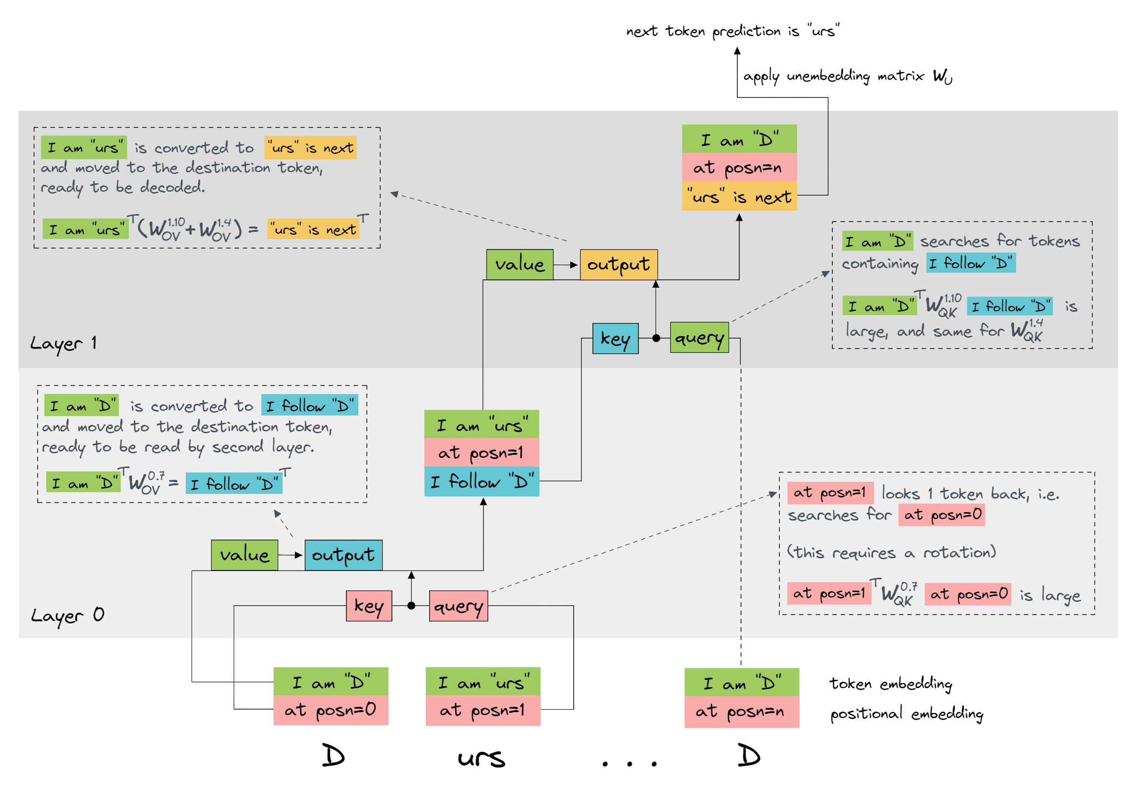
My summary of the algorithm
- Head
0.7is a previous token head (the QK-circuit ensures it always attends to the previous token). - The OV circuit of head
0.7writes a copy of the previous token in a different subspace to the one used by the embedding. - The output of head
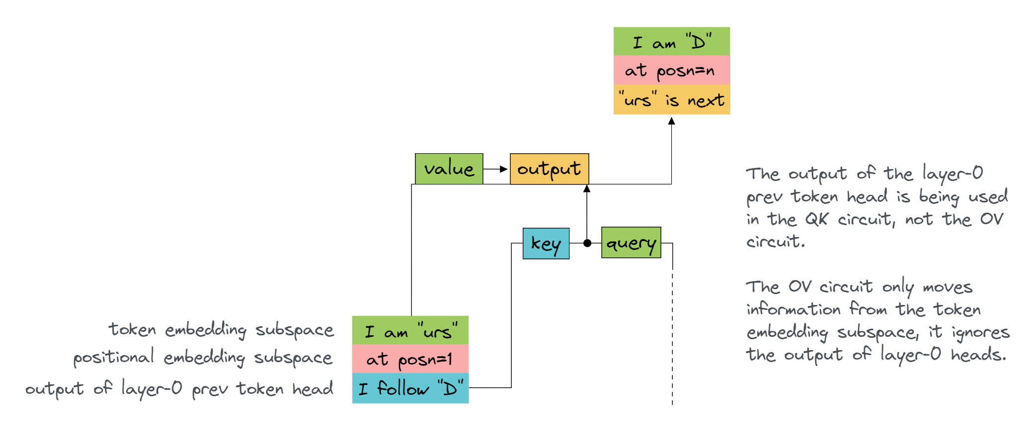
0.7is used by the key input of head1.10via K-Composition to attend to 'the source token whose previous token is the destination token'. - The OV-circuit of head
1.10copies the value of the source token to the same output logit.- Note that this is copying from the embedding subspace, not the
0.7output subspace - it is not using V-Composition at all.
- Note that this is copying from the embedding subspace, not the
1.4is also performing the same role as1.10(so together they can be more accurate - we'll see exactly how later).
To emphasise - the sophisticated hard part is computing the attention pattern of the induction head - this takes careful composition. The previous token and copying parts are fairly easy. This is a good illustrative example of how the QK circuits and OV circuits act semi-independently, and are often best thought of somewhat separately. And that computing the attention patterns can involve real and sophisticated computation!
Below is a diagram of the induction circuit, with the heads indicated in the weight matrices.
Refresher - QK and OV circuits
Before we start, a brief terminology note. I'll refer to weight matrices for a particular layer and head using superscript notation, e.g. $W_Q^{1.4}$ is the query matrix for the 4th head in layer 1, and it has shape [d_model, d_head] (remember that we multiply with weight matrices on the right). Similarly, attention patterns will be denoted $A^{1.4}$ (remember that these are activations, not parameters, since they're given by the formula $A^h = x W_{QK}^h x^T$, where $x$ is the residual stream (with shape [seq_len, d_model]).
As a shorthand, I'll often have $A$ denote the one-hot encoding of token A (i.e. the vector with zeros everywhere except a one at the index of A), so $A^T W_E$ is the embedding vector for A.
Lastly, I'll refer to special matrix products as follows:
- $W_{OV}^{h} := W_V^{h}W_O^{h}$ is the OV circuit for head $h$, and $W_E W_{OV}^h W_U$ is the full OV circuit.
- $W_{QK}^h := W_Q^h (W_K^h)^T$ is the QK circuit for head $h$, and $W_E W_{QK}^h W_E^T$ is the full QK circuit.
Note that the order of these matrices are slightly different from the Mathematical Frameworks paper - this is a consequence of the way TransformerLens stores its weight matrices.
Question - what is the interpretation of each of the following matrices?
There are quite a lot of questions here, but they are conceptually important. If you're confused, you might want to read the answers to the first few questions and then try the later ones.
In your answers, you should describe the type of input it takes, and what the outputs represent.
$W_{OV}^{h}$
Answer
$W_{OV}^{h}$ has size $(d_\text{model}, d_\text{model})$, it is a linear map describing what information gets moved from source to destination, in the residual stream.
In other words, if $x$ is a vector in the residual stream, then $x^T W_{OV}^{h}$ is the vector written to the residual stream at the destination position, if the destination token only pays attention to the source token at the position of the vector $x$.
$W_E W_{OV}^h W_U$
If $A$ is the one-hot encoding for token $W_E W_{OV}^h W_U$ has size $(d_\text{vocab}, d_\text{vocab})$, it is a linear map describing what information gets moved from source to destination, in a start-to-end sense. If $A$ is the one-hot encoding for token Hint
A (i.e. the vector with zeros everywhere except for a one in the position corresponding to token A), then think about what $A^T W_E W_{OV}^h W_U$ represents. You can evaluate this expression from left to right (e.g. start with thinking about what $A^T W_E$ represents, then multiply by the other two matrices).Answer
A, then:
A.A.
$W_{QK}^{h}$
Answer
$W_{QK}^{h}$ has size $(d_\text{model}, d_\text{model})$, it is a bilinear form describing where information is moved to and from in the residual stream (i.e. which residual stream vectors attend to which others).
$x_i^T W_{QK}^h x_j = (x_i^T W_Q^h) (x_j^T W_K^h)^T$ is the attention score paid by token $i$ to token $j$.
$W_E W_{QK}^h W_E^T$
Answer
$W_E W_{QK}^h W_E^T$ has size $(d_\text{vocab}, d_\text{vocab})$, it is a bilinear form describing where information is moved to and from, among words in our vocabulary (i.e. which tokens pay attention to which others).
If $A$ and $B$ are one-hot encodings for tokens A and B, then $A^T W_E W_{QK}^h W_E^T B$ is the attention score paid by token A to token B:
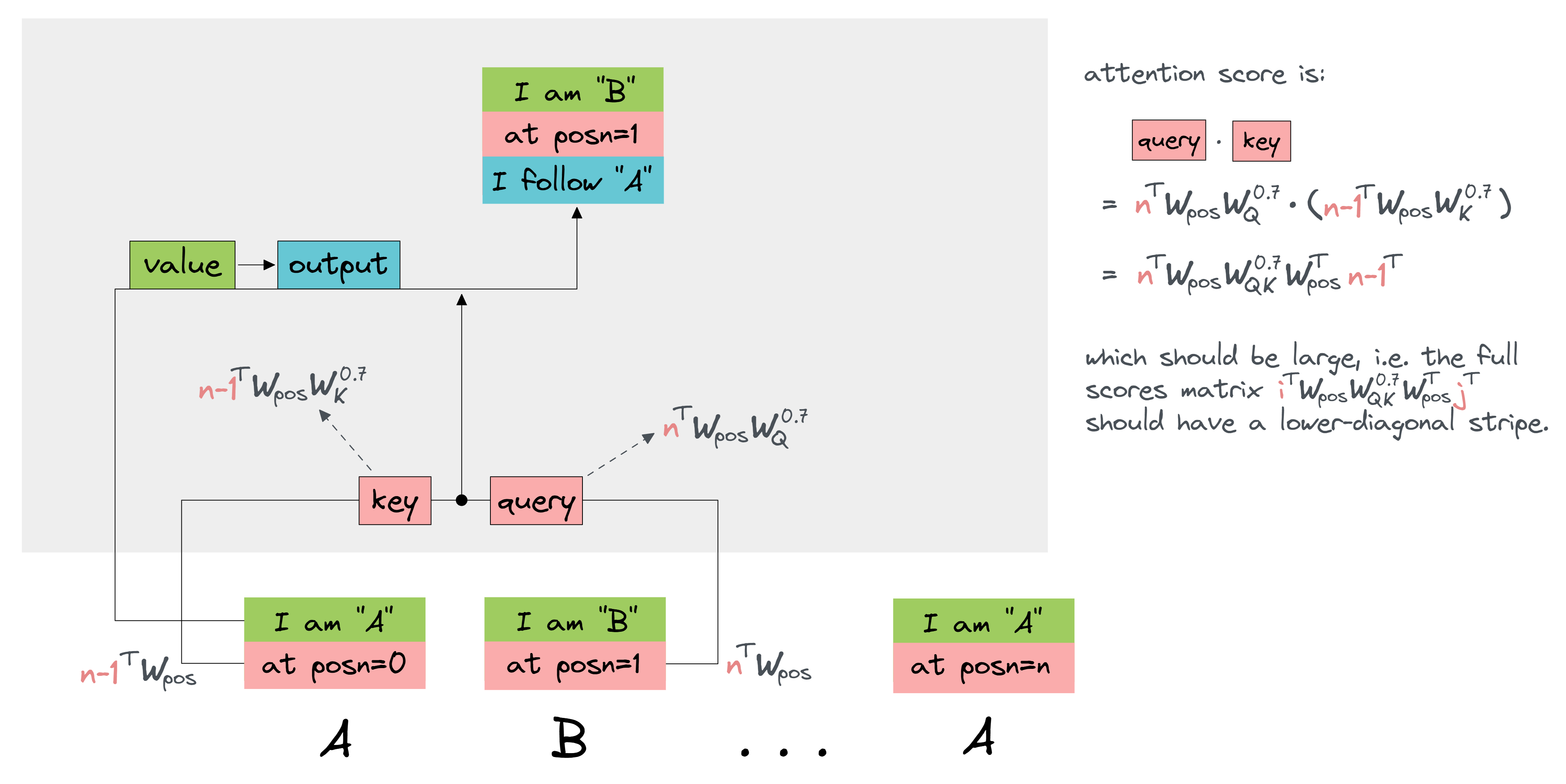
$W_{pos} W_{QK}^h W_{pos}^T$
Answer
$W_{pos} W_{QK}^h W_{pos}^T$ has size $(n_\text{ctx}, n_\text{ctx})$, it is a bilinear form describing where information is moved to and from, among tokens in our context (i.e. which token positions pay attention to other positions).
If $i$ and $j$ are one-hot encodings for positions i and j (in other words they are just the ith and jth basis vectors), then $i^T W_{pos} W_{QK}^h W_{pos}^T j$ is the attention score paid by the token with position i to the token with position j:
$W_E W_{OV}^{h_1} W_{QK}^{h_2} W_E^T$
where $h_1$ is in an earlier layer than $h_2$.
Hint
This matrix is best seen as a bilinear form of size $(d_\text{vocab}, d_\text{vocab})$. The $(A, B)$-th element is:
Answer
$W_E W_{OV}^{h_1} W_{QK}^{h_2} W_E^T$ has size $(d_\text{vocab}, d_\text{vocab})$, it is a bilinear form describing where information is moved to and from in head $h_2$, given that the query-side vector is formed from the output of head $h_1$. In other words, this is an instance of Q-composition.
If $A$ and $B$ are one-hot encodings for tokens A and B, then $A^T W_E W_{OV}^{h_1} W_{QK}^{h_2} W_E^T B$ is the attention score paid to token B, by any token which attended strongly to an A-token in head $h_1$.
To further break this down, if it still seems confusing:
Note that the actual attention score will be a sum of multiple terms, not just this one (in fact, we'd have a different term for every combination of query and key input). But this term describes the particular contribution to the attention score from this combination of query and key input, and it might be the case that this term is the only one that matters (i.e. all other terms don't much affect the final probabilities). We'll see something exactly like this later on.
Before we start, there's a problem that we might run into when calculating all these matrices. Some of them are massive, and might not fit on our GPU. For instance, both full circuit matrices have shape $(d_\text{vocab}, d_\text{vocab})$, which in our case means $50278\times 50278 \approx 2.5\times 10^{9}$ elements. Even if your GPU can handle this, it still seems inefficient. Is there any way we can meaningfully analyse these matrices, without actually having to calculate them?
Factored Matrix class
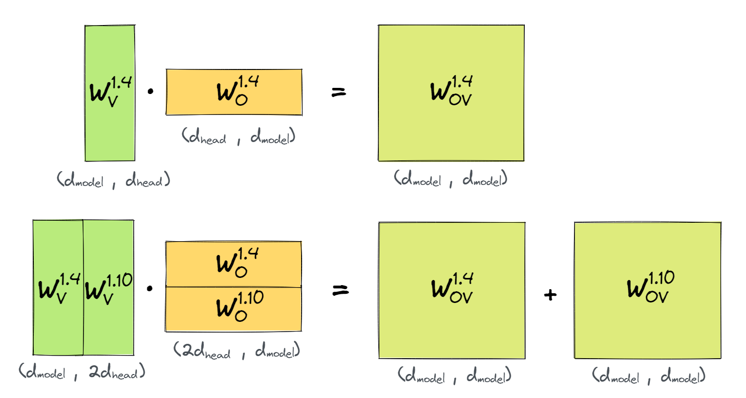
In transformer interpretability, we often need to analyse low rank factorized matrices - a matrix $M = AB$, where M is [large, large], but A is [large, small] and B is [small, large]. This is a common structure in transformers.
For instance, we can factorise the OV circuit above as $W_{OV}^h = W_V^h W_O^h$, where $W_V^h$ has shape [768, 64] and $W_O^h$ has shape [64, 768]. For an even more extreme example, the full OV circuit can be written as $(W_E W_V^h) (W_O^h W_U)$, where these two matrices have shape [50278, 64] and [64, 50278] respectively. Similarly, we can write the full QK circuit as $(W_E W_Q^h) (W_E W_K^h)^T$.
The FactoredMatrix class is a convenient way to work with these. It implements efficient algorithms for various operations on these, such as computing the trace, eigenvalues, Frobenius norm, singular value decomposition, and products with other matrices. It can (approximately) act as a drop-in replacement for the original matrix.
This is all possible because knowing the factorisation of a matrix gives us a much easier way of computing its important properties. Intuitively, since $M=AB$ is a very large matrix that operates on very small subspaces, we shouldn't expect knowing the actual values $M_{ij}$ to be the most efficient way of storing it!
Exercise - deriving properties of a factored matrix
To give you an idea of what kinds of properties you can easily compute if you have a factored matrix, let's try and derive some ourselves.
Suppose we have $M=AB$, where $A$ has shape $(m, n)$, $B$ has shape $(n, m)$, and $m > n$. So $M$ is a size-$(m, m)$ matrix with rank at most $n$.
Question - how can you easily compute the trace of $M$?
Answer
We have:
so evaluation of the trace is $O(mn)$.
Note that, by cyclicity of the trace, we can also show that $\text{Tr}(M) = \text{Tr}(BA)$ (although we don't even need to calculate the product $AB$ to evaluate the trace).
Question - how can you easily compute the eigenvalues of $M$?
(As you'll see in later exercises, eigenvalues are very important for evaluating matrices, for instance we can assess the copying scores of an OV circuit by looking at the eigenvalues of $W_{OV}$.)
It's computationally cheaper to find the eigenvalues of $BA$ rather than $AB$. How are the eigenvalues of $AB$ and $BA$ related? The eigenvalues of $AB$ and $BA$ are related as follows: if $\mathbf{v}$ is an eigenvector of $AB$ with $ABv = \lambda \mathbf{v}$, then $B\mathbf{v}$ is an eigenvector of $BA$ with the same eigenvalue:Hint
Answer
This only fails when $B\mathbf{v} = \mathbf{0}$, but in this case $AB\mathbf{v} = \mathbf{0}$ so $\lambda = 0$. Thus, we can conclude that any non-zero eigenvalues of $AB$ are also eigenvalues of $BA$.
It's much computationally cheaper to compute the eigenvalues of $BA$ (since it's a much smaller matrix), and this gives us all the non-zero eigenvalues of $AB$.
Question (hard) - how can you easily compute the SVD of $M$?
Hint
For a size-$(m, n)$ matrix with $m > n$, the algorithmic complexity of finding SVD is $O(mn^2)$. So it's relatively cheap to find the SVD of $A$ and $B$ (complexity $mn^2$ vs $m^3$). Can you use that to find the SVD of $M$?
Answer
It's much cheaper to compute the SVD of the small matrices $A$ and $B$. Denote these SVDs by:
where $U_A$ and $V_B$ are $(m, n)$, and the other matrices are $(n, n)$.
Then we have:
Note that the matrix in the middle has size $(n, n)$ (i.e. small), so we can compute its SVD cheaply:
and finally, this gives us the SVD of $M$:
where $U = U_A U'$, $V = V_B V'$, and $S = S'$.
All our SVD calculations and matrix multiplications had complexity at most $O(mn^2)$, which is much better than $O(m^3)$ (remember that we don't need to compute all the values of $U = U_A U'$, only the ones which correspond to non-zero singular values).
If you're curious, you can go to the FactoredMatrix documentation to see the implementation of the SVD calculation, as well as other properties and operations.
Now that we've discussed some of the motivations behind having a FactoredMatrix class, let's see it in action.
Basic Examples
We can use the basic class directly - let's make a factored matrix directly and look at the basic operations:
A = t.randn(5, 2)
B = t.randn(2, 5)
AB = A @ B
AB_factor = FactoredMatrix(A, B)
print("Norms:")
print(AB.norm())
print(AB_factor.norm())

print(f"Right dim: {AB_factor.rdim}, Left dim: {AB_factor.ldim}, Hidden dim: {AB_factor.mdim}")
We can also look at the eigenvalues and singular values of the matrix. Note that, because the matrix is rank 2 but 5 by 5, the final 3 eigenvalues and singular values are zero - the factored class omits the zeros.
print("Eigenvalues:")
print(t.linalg.eig(AB).eigenvalues)
print(AB_factor.eigenvalues)

print("\nSingular Values:")
print(t.linalg.svd(AB).S)
print(AB_factor.S)

print("\nFull SVD:")
print(AB_factor.svd())
Aside - the sizes of objects returned by the SVD method.
If $M = USV^T$, and M.shape = (m, n) and the rank is r, then the SVD method returns the matrices $U, S, V$. They have shape (m, r), (r,), and (n, r) respectively, because:
- We don't bother storing the off-diagonal entries of $S$, since they're all zero.
- We don't bother storing the columns of $U$ and $V$ which correspond to zero singular values, since these won't affect the value of $USV^T$.
We can multiply a factored matrix with an unfactored matrix to get another factored matrix (as in example below). We can also multiply two factored matrices together to get another factored matrix.
C = t.randn(5, 300)
ABC = AB @ C
ABC_factor = AB_factor @ C

print(f"Unfactored: shape={ABC.shape}, norm={ABC.norm()}")
print(f"Factored: shape={ABC_factor.shape}, norm={ABC_factor.norm()}")
print(f"\nRight dim: {ABC_factor.rdim}, Left dim: {ABC_factor.ldim}, Hidden dim: {ABC_factor.mdim}")
If we want to collapse this back to an unfactored matrix, we can use the AB property to get the product:
AB_unfactored = AB_factor.AB
t.testing.assert_close(AB_unfactored, AB)
Reverse-engineering circuits
Within our induction circuit, we have four individual circuits: the OV and QK circuits in our previous token head, and the OV and QK circuits in our induction head. In the following sections of the exercise, we'll reverse-engineer each of these circuits in turn.
- In the section OV copying circuit, we'll look at the layer-1 OV circuit.
- In the section QK prev-token circuit, we'll look at the layer-0 QK circuit.
- The third section (K-composition) is a bit trickier, because it involves looking at the composition of the layer-0 OV circuit and layer-1 QK circuit. We will have to do two things:
- Show that these two circuits are composing (i.e. that the output of the layer-0 OV circuit is the main determinant of the key vectors in the layer-1 QK circuit).
- Show that the joint operation of these two circuits is "make the second instance of a token attend to the token following an earlier instance.
The dropdown below contains a diagram explaining how the three sections relate to the different components of the induction circuit. You might have to open it in a new tab to see it clearly.
Diagram
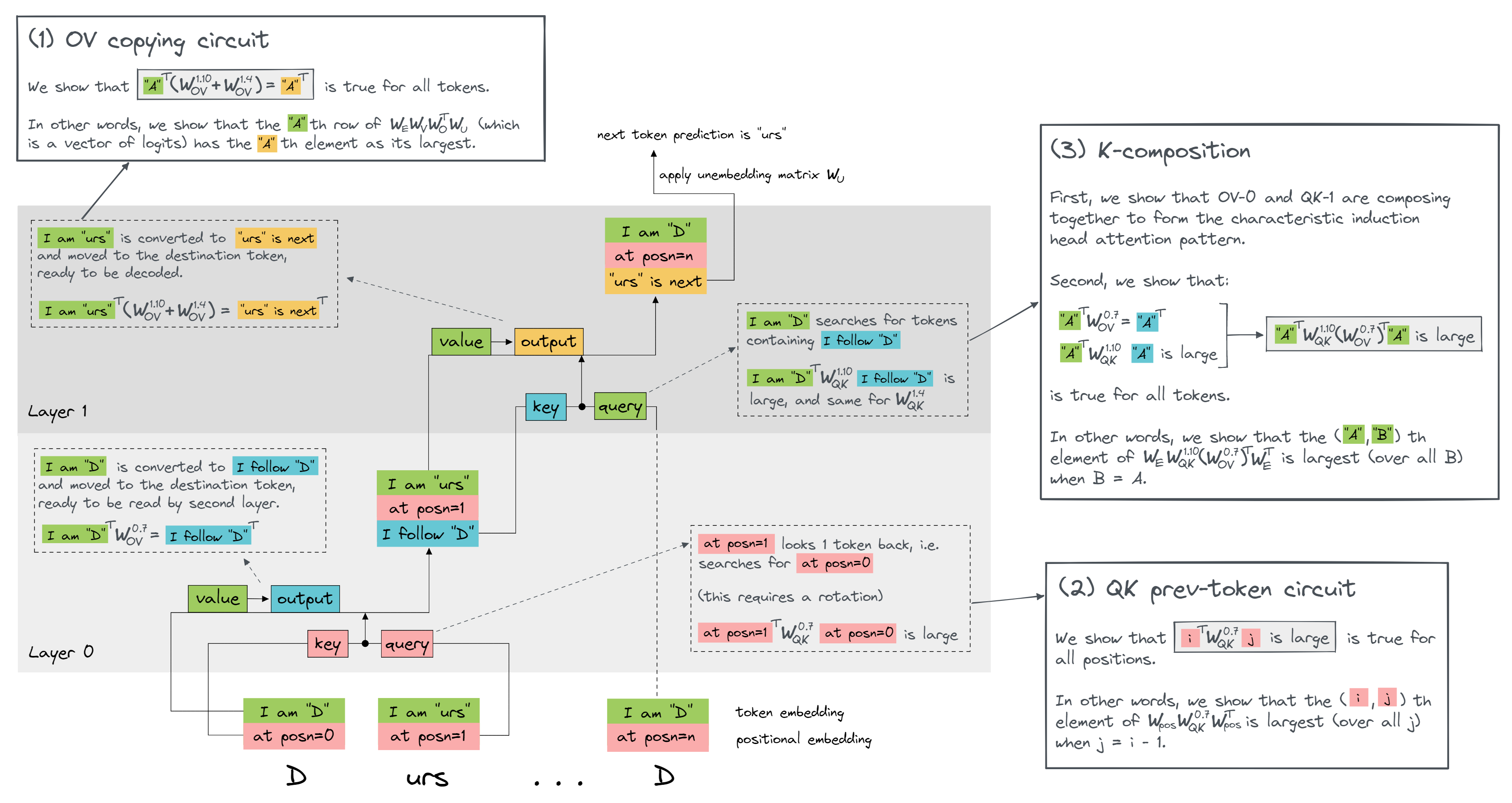
After this, we'll have a look at composition scores, which are a more mathematically justified way of showing that two attention heads are composing (without having to look at their behaviour on any particular class of inputs, since it is a property of the actual model weights).
[1] OV copying circuit
Let's start with an easy parts of the circuit - the copying OV circuit of 1.4 and 1.10. Let's start with head 4. The only interpretable (read: privileged basis) things here are the input tokens and output logits, so we want to study the matrix:
(and same for 1.10). This is the $(d_\text{vocab}, d_\text{vocab})$-shape matrix that combines with the attention pattern to get us from input to output.
We want to calculate this matrix, and inspect it. We should find that its diagonal values are very high, and its non-diagonal values are much lower.
Question - why should we expect this observation? (you may find it helpful to refer back to the previous section, where you described what the interpretation of different matrices was.)
Hint
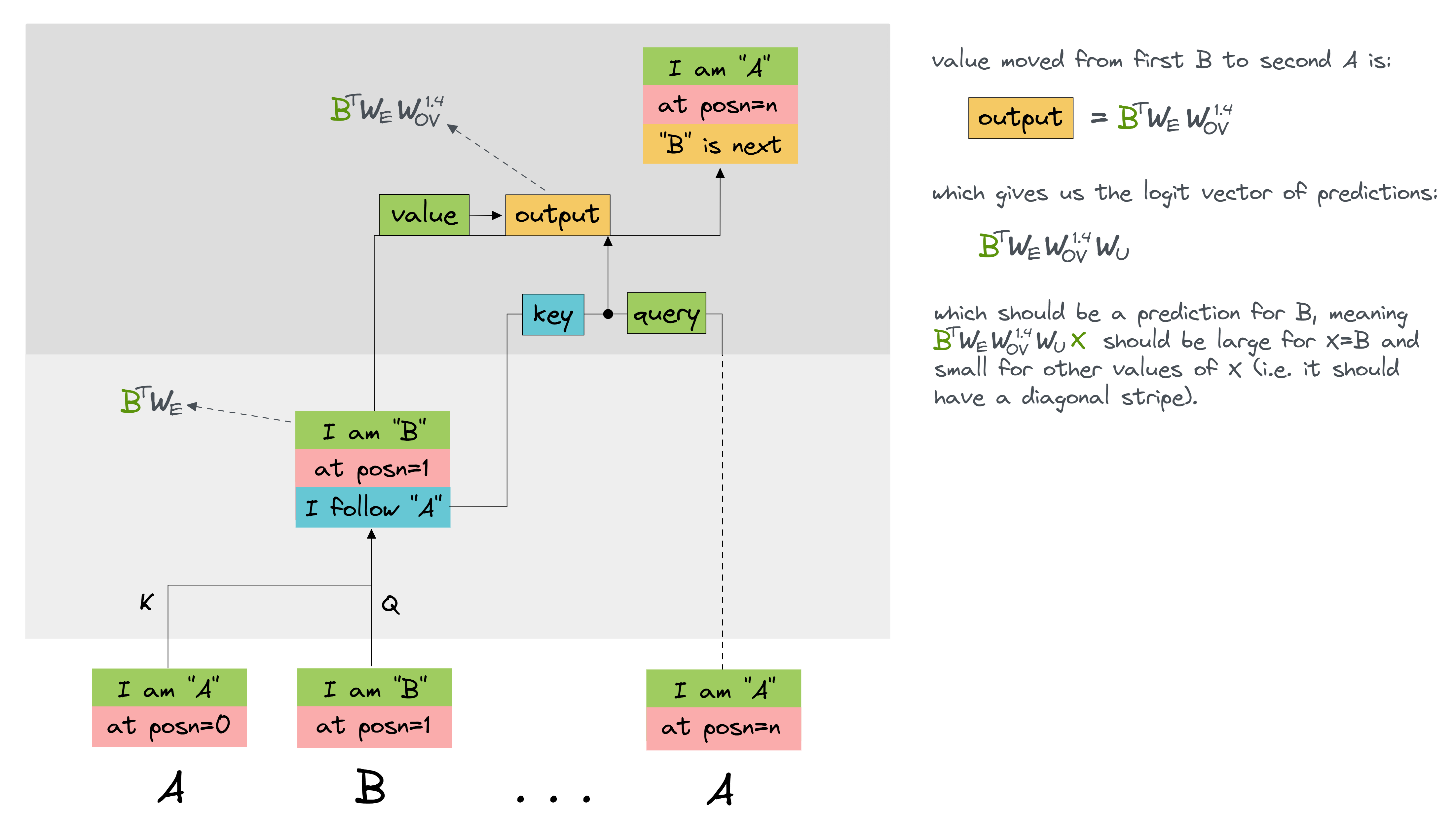
Suppose our repeating sequence is A B ... A B. Let $A$, $B$ be the corresponding one-hot encoded tokens. The B-th row of this matrix is:
What is the interpretation of this expression, in the context of our attention head?
Answer
If our repeating sequence is A B ... A B, then:
is the vector of logits which gets moved from the first B token to the second A token, to be used as the prediction for the token following the second A token. It should result in a high prediction for B, and a low prediction for everything else. In other words, the (B, X)-th element of this matrix should be highest for X=B, which is exactly what we claimed.
If this still seems confusing, the diagram below might help:
Exercise - compute OV circuit for 1.4
This is the first of several similar exercises where you calculate a circuit by multiplying matrices. This exercise is pretty important (in particular, you should make sure you understand what this matrix represents and why we're interested in it), but the actual calculation shouldn't take very long.
You should compute it as a FactoredMatrix object.
Remember, you can access the model's weights directly e.g. using model.W_E or model.W_Q (the latter gives you all the W_Q matrices, indexed by layer and head).
head_index = 4
layer = 1

# YOUR CODE HERE - complete the `full_OV_circuit` object

tests.test_full_OV_circuit(full_OV_circuit, model, layer, head_index)
Help - I'm not sure how to use this class to compute a product of more than 2 matrices.
You can compute it directly, as:
full_OV_circuit = FactoredMatrix(W_E @ W_V, W_O @ W_U)
Alternatively, another nice feature about the FactoredMatrix class is that you can chain together matrix multiplications. The following code defines exactly the same FactoredMatrix object:
OV_circuit = FactoredMatrix(W_V, W_O)
full_OV_circuit = W_E @ OV_circuit @ W_U
Solution
head_index = 4
layer = 1

W_O = model.W_O[layer, head_index]
W_V = model.W_V[layer, head_index]
W_E = model.W_E
W_U = model.W_U

OV_circuit = FactoredMatrix(W_V, W_O)
full_OV_circuit = W_E @ OV_circuit @ W_U
Now we want to check that this matrix is the identity. Since it's in factored matrix form, this is a bit tricky, but there are still things we can do.
First, to validate that it looks diagonal-ish, let's pick 200 random rows and columns and visualise that - it should at least look identity-ish here! We're using the indexing method of the FactoredMatrix class - you can index into it before returning the actual .AB value, to avoid having to compute the whole thing (we take advantage of the fact that A[left_indices, :] @ B[:, right_indices] is the same as (A @ B)[left_indices, right_indices]).
indices = t.randint(0, model.cfg.d_vocab, (200,))
full_OV_circuit_sample = full_OV_circuit[indices, indices].AB

imshow(
    full_OV_circuit_sample,
    labels={"x": "Logits on output token", "y": "Input token"},
    title="Full OV circuit for copying head",
    width=700,
    height=600,
)
Click to see the expected output
Aside - indexing factored matrices
Yet another nice thing about factored matrices is that you can evaluate small submatrices without having to compute the entire matrix. This is based on the fact that the [i, j]-th element of matrix AB is A[i, :] @ B[:, j].
Exercise - compute circuit accuracy
When you index a factored matrix, you get back another factored matrix. So rather than explicitly calculating A[left_indices, :] @ B[:, left_indices], we can just write AB[left_indices, left_indices].
You should observe a pretty distinct diagonal pattern here, which is a good sign. However, the matrix is pretty noisy so it probably won't be exactly the identity. Instead, we should come up with a summary statistic to capture a rough sense of "closeness to the identity".
Accuracy is a good summary statistic - what fraction of the time is the largest logit on the diagonal? Even if there's lots of noise, you'd probably still expect the largest logit to be on the diagonal a good deal of the time.
If you're on a Colab or have a powerful GPU, you should be able to compute the full matrix and perform this test. However, it's better practice to iterate through this matrix when we can, so that we avoid CUDA issues. We've given you a batch_size argument in the function below, and you should try to only explicitly calculate matrices of size batch_size * d_vocab rather than the massive matrix of d_vocab * d_vocab.
def top_1_acc(full_OV_circuit: FactoredMatrix, batch_size: int = 1000) -> float:
    """
    Return the fraction of the time that the maximum value is on the circuit diagonal.
    """
    raise NotImplementedError()


print(f"Fraction of time that the best logit is on diagonal: {top_1_acc(full_OV_circuit):.4f}")
Help - I'm not sure whether to take the argmax over rows or columns.
The OV circuit is defined as W_E @ W_OV @ W_U. We can see the i-th row W_E[i] @ W_OV @ W_U as the vector representing the logit vector added at any token which attends to the i-th token, via the attention head with OV matrix W_OV.
So we want to take the argmax over rows (i.e. over dim=1), because we're interested in the number of tokens tok in the vocabulary such that when tok is attended to, it is also the top prediction.
Solution
def top_1_acc(full_OV_circuit: FactoredMatrix, batch_size: int = 1000) -> float:
    """
    Return the fraction of the time that the maximum value is on the circuit diagonal.
    """
    total = 0

    for indices in t.split(t.arange(full_OV_circuit.shape[0], device=device), batch_size):
        AB_slice = full_OV_circuit[indices].AB
        total += (t.argmax(AB_slice, dim=1) == indices).float().sum().item()

    return total / full_OV_circuit.shape[0]
This should return about 30.79% - pretty underwhelming. It goes up to 47.73% for top-5, but still not great. What's up with that?
Exercise - compute effective circuit
Now we return to why we have two induction heads. If both have the same attention pattern, the effective OV circuit is actually $W_E(W_V^{1.4}W_O^{1.4}+W_V^{1.10}W_O^{1.10})W_U$, and this is what matters. So let's re-run our analysis on this!
Question - why might the model want to split the circuit across two heads?
Because $W_V W_O$ is a rank 64 matrix. The sum of two is a rank 128 matrix. This can be a significantly better approximation to the desired 50K x 50K matrix!
# YOUR CODE HERE - compute the effective OV circuit, and run `top_1_acc` on it
Expected output
You should get an accuracy of 95.6% for top-1 - much better!
Note that you can also try top 5 accuracy, which improves your result to 98%.
Solution
W_O_both = einops.rearrange(model.W_O[1, [4, 10]], "head d_head d_model -> (head d_head) d_model")
W_V_both = einops.rearrange(model.W_V[1, [4, 10]], "head d_model d_head -> d_model (head d_head)")

W_OV_eff = W_E @ FactoredMatrix(W_V_both, W_O_both) @ W_U

print(f"Fraction of the time that the best logit is on the diagonal: {top_1_acc(W_OV_eff):.4f}")
[2] QK prev-token circuit
The other easy circuit is the QK-circuit of L0H7 - how does it know to be a previous token circuit?
We can multiply out the full QK circuit via the positional embeddings:
to get a matrix pos_by_pos of shape [max_ctx, max_ctx] (max ctx = max context length, i.e. maximum length of a sequence we're allowing, which is set by our choice of dimensions in $W_\text{pos}$).
Note that in this case, our max context window is 2048 (we can check this via model.cfg.n_ctx). This is much smaller than the 50k-size matrices we were working with in the previous section, so we shouldn't need to use the factored matrix class here.
Exercise - interpret full QK-circuit for 0.7
The code below plots the full QK circuit for head 0.7 (including a scaling and softmax step, which is meant to mirror how the QK bilinear form will be used in actual attention layers). You should run the code, and interpret the results in the context of the induction circuit.
layer = 0
head_index = 7

# Compute full QK matrix (for positional embeddings)
W_pos = model.W_pos
W_QK = model.W_Q[layer, head_index] @ model.W_K[layer, head_index].T
pos_by_pos_scores = W_pos @ W_QK @ W_pos.T

# Mask, scale and softmax the scores
mask = t.tril(t.ones_like(pos_by_pos_scores)).bool()
pos_by_pos_pattern = t.where(mask, pos_by_pos_scores / model.cfg.d_head**0.5, -1.0e6).softmax(-1)

# Plot the results
print(f"Avg lower-diagonal value: {pos_by_pos_pattern.diag(-1).mean():.4f}")
imshow(
    utils.to_numpy(pos_by_pos_pattern[:200, :200]),
    labels={"x": "Key", "y": "Query"},
    title="Attention patterns for prev-token QK circuit, first 100 indices",
    width=700,
    height=600,
)
Click to see the expected output (and interpretation)
Avg lower-diagonal value: 0.9978
The full QK circuit $W_\text{pos} W_{QK}^{0.7} W_\text{pos}^T$ has shape [n_ctx, n_ctx]. It is a bilinear form, with the $(i, j)$-th element representing the attention score paid by the $i$-th token to the $j$-th token. This should be very large when $j = i - 1$ (and smaller for all other values of $j$), because this is a previous head token. So if we softmax over $j$, we should get a lower-diagonal stripe of 1.
Why is it justified to ignore token encodings? In this case, it turns out that the positional encodings have a much larger effect on the attention scores than the token encodings. If you want, you can verify this for yourself - after going through the next section (reverse-engineering K-composition), you'll have a better sense of how to perform attribution on the inputs to attention heads, and assess their importance.
[3] K-composition circuit
We now dig into the hard part of the circuit - demonstrating the K-Composition between the previous token head and the induction head.
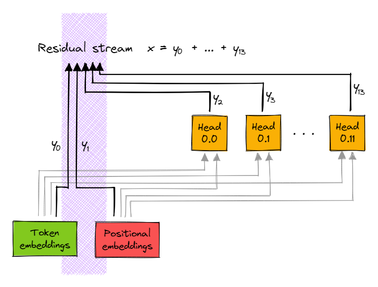
Splitting activations
We can repeat the trick from the logit attribution scores. The QK-input for layer 1 is the sum of 14 terms (2+n_heads) - the token embedding, the positional embedding, and the results of each layer 0 head. So for each head $\text{H}$ in layer 1, the query tensor (ditto key) corresponding to sequence position $i$ is:
where $e$ stands for the token embedding, $pe$ for the positional embedding, and $x^\text{0.h}$ for the output of head $h$ in layer 0 (and the sum of these tensors equals the residual stream $x$). All these tensors have shape [seq, d_model]. So we can treat the expression above as a sum of matrix multiplications [seq, d_model] @ [d_model, d_head] -> [seq, d_head].
For ease of notation, I'll refer to the 14 inputs as $(y_0, y_1, ..., y_{13})$ rather than $(e, pe, x^\text{0.h}, ..., x^{h.11})$. So we have:
with each $y_i$ having shape [seq, d_model], and the sum of $y_i$s being the full residual stream $x$. Here is a diagram to illustrate:
Exercise - analyse the relative importance
We can now analyse the relative importance of these 14 terms! A very crude measure is to take the norm of each term (by component and position).
Note that this is a pretty dodgy metric - q and k are not inherently interpretable! But it can be a good and easy-to-compute proxy.
Question - why are Q and K not inherently interpretable? Why might the norm be a good metric in spite of this?
They are not inherently interpretable because they operate on the residual stream, which doesn't have a privileged basis. You could stick a rotation matrix $R$ after all of the $Q$, $K$ and $V$ weights (and stick a rotation matrix before everything that writes to the residual stream), and the model would still behave exactly the same.
The reason taking the norm is still a reasonable thing to do is that, despite the individual elements of these vectors not being inherently interpretable, it's still a safe bet that if they are larger than they will have a greater overall effect on the residual stream. So looking at the norm doesn't tell us how they work, but it does indicate which ones are more important.
Fill in the functions below:
def decompose_qk_input(cache: ActivationCache) -> Float[Tensor, "n_heads+2 posn d_model"]:
    """
    Retrieves all the input tensors to the first attention layer, and concatenates them along the
    0th dim.

    The [i, :, :]th element is y_i (from notation above). The sum of these tensors along the 0th
    dim should be the input to the first attention layer.
    """
    raise NotImplementedError()


def decompose_q(
    decomposed_qk_input: Float[Tensor, "n_heads+2 posn d_model"],
    ind_head_index: int,
    model: HookedTransformer,
) -> Float[Tensor, "n_heads+2 posn d_head"]:
    """
    Computes the tensor of query vectors for each decomposed QK input.

    The [i, :, :]th element is y_i @ W_Q (so the sum along axis 0 is just the q-values).
    """
    raise NotImplementedError()


def decompose_k(
    decomposed_qk_input: Float[Tensor, "n_heads+2 posn d_model"],
    ind_head_index: int,
    model: HookedTransformer,
) -> Float[Tensor, "n_heads+2 posn d_head"]:
    """
    Computes the tensor of key vectors for each decomposed QK input.

    The [i, :, :]th element is y_i @ W_K(so the sum along axis 0 is just the k-values)
    """
    raise NotImplementedError()


# Recompute rep tokens/logits/cache, if we haven't already
seq_len = 50
batch_size = 1
(rep_tokens, rep_logits, rep_cache) = run_and_cache_model_repeated_tokens(model, seq_len, batch_size)
rep_cache.remove_batch_dim()

ind_head_index = 4

# First we get decomposed q and k input, and check they're what we expect
decomposed_qk_input = decompose_qk_input(rep_cache)
decomposed_q = decompose_q(decomposed_qk_input, ind_head_index, model)
decomposed_k = decompose_k(decomposed_qk_input, ind_head_index, model)
t.testing.assert_close(
    decomposed_qk_input.sum(0),
    rep_cache["resid_pre", 1] + rep_cache["pos_embed"],
    rtol=0.01,
    atol=1e-05,
)
t.testing.assert_close(decomposed_q.sum(0), rep_cache["q", 1][:, ind_head_index], rtol=0.01, atol=0.001)
t.testing.assert_close(decomposed_k.sum(0), rep_cache["k", 1][:, ind_head_index], rtol=0.01, atol=0.01)

# Second, we plot our results
component_labels = ["Embed", "PosEmbed"] + [f"0.{h}" for h in range(model.cfg.n_heads)]
for decomposed_input, name in [(decomposed_q, "query"), (decomposed_k, "key")]:
    imshow(
        utils.to_numpy(decomposed_input.pow(2).sum([-1])),
        labels={"x": "Position", "y": "Component"},
        title=f"Norms of components of {name}",
        y=component_labels,
        width=800,
        height=400,
    )
What you should see
You should see that the most important query components are the token and positional embeddings. The most important key components are those from $y_9$, which is $x_7$, i.e. from head 0.7.
A technical note on the positional embeddings - optional, feel free to skip this.
You might be wondering why the tests compare the decomposed qk sum with the sum of the resid_pre + pos_embed, rather than just resid_pre. The answer lies in how we defined the transformer, specifically in this line from the config:
positional_embedding_type="shortformer"
The result of this is that the positional embedding isn't added to the residual stream. Instead, it's added as inputs to the Q and K calculation (i.e. we calculate (resid_pre + pos_embed) @ W_Q and same for W_K), but not as inputs to the V calculation (i.e. we just calculate resid_pre @ W_V). This isn't actually how attention works in general, but for our purposes it makes the analysis of induction heads cleaner because we don't have positional embeddings interfering with the OV circuit.
Question - this type of embedding actually makes it impossible for attention heads to form via Q-composition. Can you see why?
Solution
def decompose_qk_input(cache: ActivationCache) -> Float[Tensor, "n_heads+2 posn d_model"]:
    """
    Retrieves all the input tensors to the first attention layer, and concatenates them along the
    0th dim.

    The [i, :, :]th element is y_i (from notation above). The sum of these tensors along the 0th
    dim should be the input to the first attention layer.
    """
    y0 = cache["embed"].unsqueeze(0)  # shape (1, seq, d_model)
    y1 = cache["pos_embed"].unsqueeze(0)  # shape (1, seq, d_model)
    y_rest = cache["result", 0].transpose(0, 1)  # shape (12, seq, d_model)

    return t.concat([y0, y1, y_rest], dim=0)


def decompose_q(
    decomposed_qk_input: Float[Tensor, "n_heads+2 posn d_model"],
    ind_head_index: int,
    model: HookedTransformer,
) -> Float[Tensor, "n_heads+2 posn d_head"]:
    """
    Computes the tensor of query vectors for each decomposed QK input.

    The [i, :, :]th element is y_i @ W_Q (so the sum along axis 0 is just the q-values).
    """
    W_Q = model.W_Q[1, ind_head_index]

    return einops.einsum(decomposed_qk_input, W_Q, "n seq d_model, d_model d_head -> n seq d_head")


def decompose_k(
    decomposed_qk_input: Float[Tensor, "n_heads+2 posn d_model"],
    ind_head_index: int,
    model: HookedTransformer,
) -> Float[Tensor, "n_heads+2 posn d_head"]:
    """
    Computes the tensor of key vectors for each decomposed QK input.

    The [i, :, :]th element is y_i @ W_K(so the sum along axis 0 is just the k-values)
    """
    W_K = model.W_K[1, ind_head_index]

    return einops.einsum(decomposed_qk_input, W_K, "n seq d_model, d_model d_head -> n seq d_head")


# Recompute rep tokens/logits/cache, if we haven't already
seq_len = 50
batch_size = 1
(rep_tokens, rep_logits, rep_cache) = run_and_cache_model_repeated_tokens(model, seq_len, batch_size)
rep_cache.remove_batch_dim()

ind_head_index = 4

# First we get decomposed q and k input, and check they're what we expect
decomposed_qk_input = decompose_qk_input(rep_cache)
decomposed_q = decompose_q(decomposed_qk_input, ind_head_index, model)
decomposed_k = decompose_k(decomposed_qk_input, ind_head_index, model)
t.testing.assert_close(
    decomposed_qk_input.sum(0),
    rep_cache["resid_pre", 1] + rep_cache["pos_embed"],
    rtol=0.01,
    atol=1e-05,
)
t.testing.assert_close(decomposed_q.sum(0), rep_cache["q", 1][:, ind_head_index], rtol=0.01, atol=0.001)
t.testing.assert_close(decomposed_k.sum(0), rep_cache["k", 1][:, ind_head_index], rtol=0.01, atol=0.01)

# Second, we plot our results
component_labels = ["Embed", "PosEmbed"] + [f"0.{h}" for h in range(model.cfg.n_heads)]
for decomposed_input, name in [(decomposed_q, "query"), (decomposed_k, "key")]:
    imshow(
        utils.to_numpy(decomposed_input.pow(2).sum([-1])),
        labels={"x": "Position", "y": "Component"},
        title=f"Norms of components of {name}",
        y=component_labels,
        width=800,
        height=400,
    )
This tells us which heads are probably important, but we can do better than that. Rather than looking at the query and key components separately, we can see how they combine together - i.e. take the decomposed attention scores.
This is a bilinear function of q and k, and so we will end up with a decomposed_scores tensor with shape [query_component, key_component, query_pos, key_pos], where summing along BOTH of the first axes will give us the original attention scores (pre-mask).
Exercise - decompose attention scores
Implement the function giving the decomposed scores (remember to scale by sqrt(d_head)!) For now, don't mask it.
Question - why do I focus on the attention scores, not the attention pattern? (i.e. pre softmax not post softmax)
Because the decomposition trick only works for things that are linear - softmax isn't linear and so we can no longer consider each component independently.
Help - I'm confused about what we're doing / why we're doing it.
Remember that each of our components writes to the residual stream separately. So after layer 0, we have:
We're particularly interested in the attention scores computed in head 1.4, and how they depend on the inputs into that head. We've already decomposed the residual stream value $x$ into its terms $e$, $pe$, and $x^ 0$ through $x^{11}$ (which we've labelled $y_0, ..., y_{13}$ for simplicity), and we've done the same for key and query terms. We can picture these terms being passed into head 1.4 as:
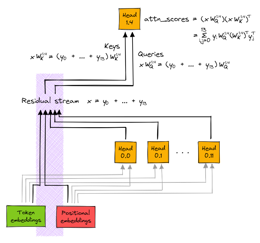
So when we expand attn_scores out in full, they are a sum of $14^2 = 196$ terms - one for each combination of (query_component, key_component).
Why is this decomposition useful?
We have a theory about a particular circuit in our model. We think that head 1.4 is an induction head, and the most important components that feed into this head are the prev token head 0.7 (as key) and the token embedding (as query). This is already supported by the evidence of our magnitude plots above (because we saw that 0.7 as key and token embeddings as query were large), but we still don't know how this particular key and query work together; we've only looked at them separately.
By decomposing attn_scores like this, we can check whether the contribution from combination (query=tok_emb, key=0.7) is indeed producing the characteristic induction head pattern which we've observed (and the other 195 terms don't really matter).
def decompose_attn_scores(
    decomposed_q: Float[Tensor, "q_comp q_pos d_head"],
    decomposed_k: Float[Tensor, "k_comp k_pos d_head"],
    model: HookedTransformer,
) -> Float[Tensor, "q_comp k_comp q_pos k_pos"]:
    """
    Output is decomposed_scores with shape [query_component, key_component, query_pos, key_pos]

    The [i, j, 0, 0]th element is y_i @ W_QK @ y_j^T (so the sum along both first axes are the
    attention scores)
    """
    raise NotImplementedError()


tests.test_decompose_attn_scores(decompose_attn_scores, decomposed_q, decomposed_k, model)
Solution
def decompose_attn_scores(
    decomposed_q: Float[Tensor, "q_comp q_pos d_head"],
    decomposed_k: Float[Tensor, "k_comp k_pos d_head"],
    model: HookedTransformer,
) -> Float[Tensor, "q_comp k_comp q_pos k_pos"]:
    """
    Output is decomposed_scores with shape [query_component, key_component, query_pos, key_pos]

    The [i, j, 0, 0]th element is y_i @ W_QK @ y_j^T (so the sum along both first axes are the
    attention scores)
    """
    return einops.einsum(
        decomposed_q,
        decomposed_k,
        "q_comp q_pos d_head, k_comp k_pos d_head -> q_comp k_comp q_pos k_pos",
    ) / (model.cfg.d_head**0.5)
Once these tests have passed, you can plot the results:
# First plot: attention score contribution from (query_component, key_component) = (Embed, L0H7), you can replace this
# with any other pair and see that the values are generally much smaller, i.e. this pair dominates the attention score
# calculation
decomposed_scores = decompose_attn_scores(decomposed_q, decomposed_k, model)

q_label = "Embed"
k_label = "0.7"
decomposed_scores_from_pair = decomposed_scores[component_labels.index(q_label), component_labels.index(k_label)]

imshow(
    utils.to_numpy(t.tril(decomposed_scores_from_pair)),
    title=f"Attention score contributions from query = {q_label}, key = {k_label}<br>(by query & key sequence positions)",
    width=700,
)


# Second plot: std dev over query and key positions, shown by component. This shows us that the other pairs of
# (query_component, key_component) are much less important, without us having to look at each one individually like we
# did in the first plot!
decomposed_stds = einops.reduce(
    decomposed_scores, "query_decomp key_decomp query_pos key_pos -> query_decomp key_decomp", t.std
)
imshow(
    utils.to_numpy(decomposed_stds),
    labels={"x": "Key Component", "y": "Query Component"},
    title="Std dev of attn score contributions across sequence positions<br>(by query & key comp)",
    x=component_labels,
    y=component_labels,
    width=700,
)
Click to see the expected output
Help - I don't understand the interpretation of these plots.
The first plot tells you that the term $e W_{QK}^{1.4} (x^{0.7})^T$ (i.e. the component of the attention scores for head 1.4 where the query is supplied by the token embeddings and the key is supplied by the output of head 0.7) produces the distinctive attention pattern we see in the induction head: a strong diagonal stripe.
Although this tells us that this this component would probably be sufficient to implement the induction mechanism, it doesn't tell us the whole story. Ideally, we'd like to show that the other 195 terms are unimportant. Taking the standard deviation across the attention scores for a particular pair of components is a decent proxy for how important this term is in the overall attention pattern. The second plot shows us that the standard deviation is very small for all the other components, so we can be confident that the other components are unimportant.
To summarise:
- The first plot tells us that the pair
(q_component=tok_emb, k_component=0.7)produces the characteristic induction-head pattern we see in attention head1.4. - The second plot confirms that this pair is the only important one for influencing the attention pattern in
1.4; all other pairs have very small contributions.
Note that plots like the ones above are often the most concise way of presenting a summary of the important information, and understanding what to plot is a valuable skill in any model internals-based work. However, if you want to see the "full plot" which the two plots above are both simplifications of in some sense, you can run the code below, which gives you the matrix of every single pair of components' contribution to the attention scores. So the first plot above is just a slice of the full plot below, and the second plot above is just the plot below after reducing over each slice with the standard deviation operation.
(Note - the plot you'll generate below is pretty big, so you'll want to clear it after you're done with it. If your machine is still working slowly when rendering it, you can use fig.show(config={"staticPlot": True}) to display a non-interactive version of it.)
decomposed_scores_centered = t.tril(decomposed_scores - decomposed_scores.mean(dim=-1, keepdim=True))

decomposed_scores_reshaped = einops.rearrange(
    decomposed_scores_centered,
    "q_comp k_comp q_token k_token -> (q_comp q_token) (k_comp k_token)",
)

fig = imshow(
    decomposed_scores_reshaped,
    title="Attention score contributions from all pairs of (key, query) components",
    width=1200,
    height=1200,
    return_fig=True,
)
full_seq_len = seq_len * 2 + 1
for i in range(0, full_seq_len * len(component_labels), full_seq_len):
    fig.add_hline(y=i, line_color="black", line_width=1)
    fig.add_vline(x=i, line_color="black", line_width=1)

fig.show(config={"staticPlot": True})
Click to see the expected output
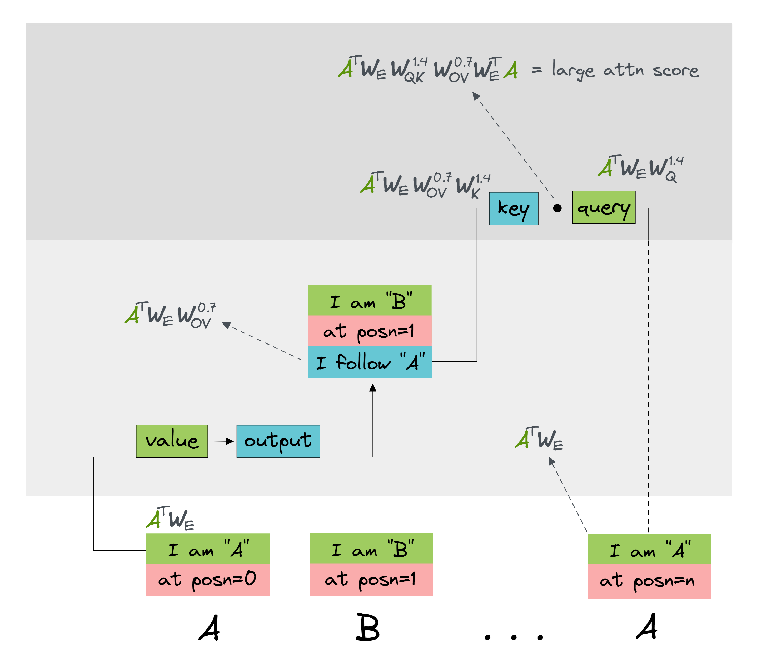
Interpreting the full circuit
Now we know that head 1.4 is composing with head 0.7 via K composition, we can multiply through to create a full circuit:
and verify that it's the identity. (Note, when we say identity here, we're again thinking about it as a distribution over logits, so this should be taken to mean "high diagonal values", and we'll be using our previous metric of top_1_acc.)
Question - why should this be the identity?
Answer
This matrix is a bilinear form. Its diagonal elements $(A, A)$ are:
Intuitively, the query is saying "I'm looking for a token which followed $A$", and the key is saying "I am a token which followed $A$" (recall that $A^T W_E W_{OV}^{0.7}$ is the vector which gets moved one position forward by our prev token head 0.7).
Now, consider the off-diagonal elements $(A, X)$ (for $X \neq A$). We expect these to be small, because the key doesn't match the query:
Hence, we expect this to be the identity.
An illustration:
Exercise - compute the K-comp circuit
Calculate the matrix above, as a FactoredMatrix object.
Aside about multiplying FactoredMatrix objects together.
If M1 = A1 @ B1 and M2 = A2 @ B2 are factored matrices, then M = M1 @ M2 returns a new factored matrix. This might be:
FactoredMatrix(M1.AB @ M2.A, M2.B)
or it might be:
FactoredMatrix(M1.A, M1.B @ M2.AB)
with these two objects corresponding to the factorisations $M = (A_1 B_1 A_2) (B_2)$ and $M = (A_1) (B_1 A_2 B_2)$ respectively.
Which one gets returned depends on the size of the hidden dimension, e.g. M1.mdim < M2.mdim then the factorisation used will be $M = A_1 B_1 (A_2 B_2)$.
Remember that both these factorisations are valid, and will give you the exact same SVD. The only reason to prefer one over the other is for computational efficiency (we prefer a smaller bottleneck dimension, because this determines the computational complexity of operations like finding SVD).
def find_K_comp_full_circuit(
    model: HookedTransformer, prev_token_head_index: int, ind_head_index: int
) -> FactoredMatrix:
    """
    Returns a (vocab, vocab)-size FactoredMatrix, with the first dimension being the query side
    (direct from token embeddings) and the second dimension being the key side (going via the
    previous token head).
    """
    raise NotImplementedError()


prev_token_head_index = 7
ind_head_index = 4
K_comp_circuit = find_K_comp_full_circuit(model, prev_token_head_index, ind_head_index)

tests.test_find_K_comp_full_circuit(find_K_comp_full_circuit, model)

print(f"Token frac where max-activating key = same token: {top_1_acc(K_comp_circuit.T):.4f}")
Solution
def find_K_comp_full_circuit(
    model: HookedTransformer, prev_token_head_index: int, ind_head_index: int
) -> FactoredMatrix:
    """
    Returns a (vocab, vocab)-size FactoredMatrix, with the first dimension being the query side
    (direct from token embeddings) and the second dimension being the key side (going via the
    previous token head).
    """
    W_E = model.W_E
    W_Q = model.W_Q[1, ind_head_index]
    W_K = model.W_K[1, ind_head_index]
    W_O = model.W_O[0, prev_token_head_index]
    W_V = model.W_V[0, prev_token_head_index]

    Q = W_E @ W_Q
    K = W_E @ W_V @ W_O @ W_K
    return FactoredMatrix(Q, K.T)
You can also try this out for our other induction head ind_head_index=10, which should also return a relatively high result. Is it higher than for head 1.4 ?
Note - unlike last time, it doesn't make sense to consider the "effective circuit" formed by adding together the weight matrices for heads 1.4 and 1.10. Can you see why?
Because the weight matrices we're dealing with here are from the QK circuit, not the OV circuit. These don't get combined in a linear way; instead we take softmax over each head's QK-circuit output individually.
Further Exploration of Induction Circuits
I now consider us to have fully reverse engineered an induction circuit - by both interpreting the features and by reverse engineering the circuit from the weights. But there's a bunch more ideas that we can apply for finding circuits in networks that are fun to practice on induction heads, so here's some bonus content - feel free to skip to the later bonus ideas though.
Composition scores
A particularly cool idea in the paper is the idea of virtual weights, or compositional scores. (Though I came up with it, so I'm deeply biased!). This is used to identify induction heads.
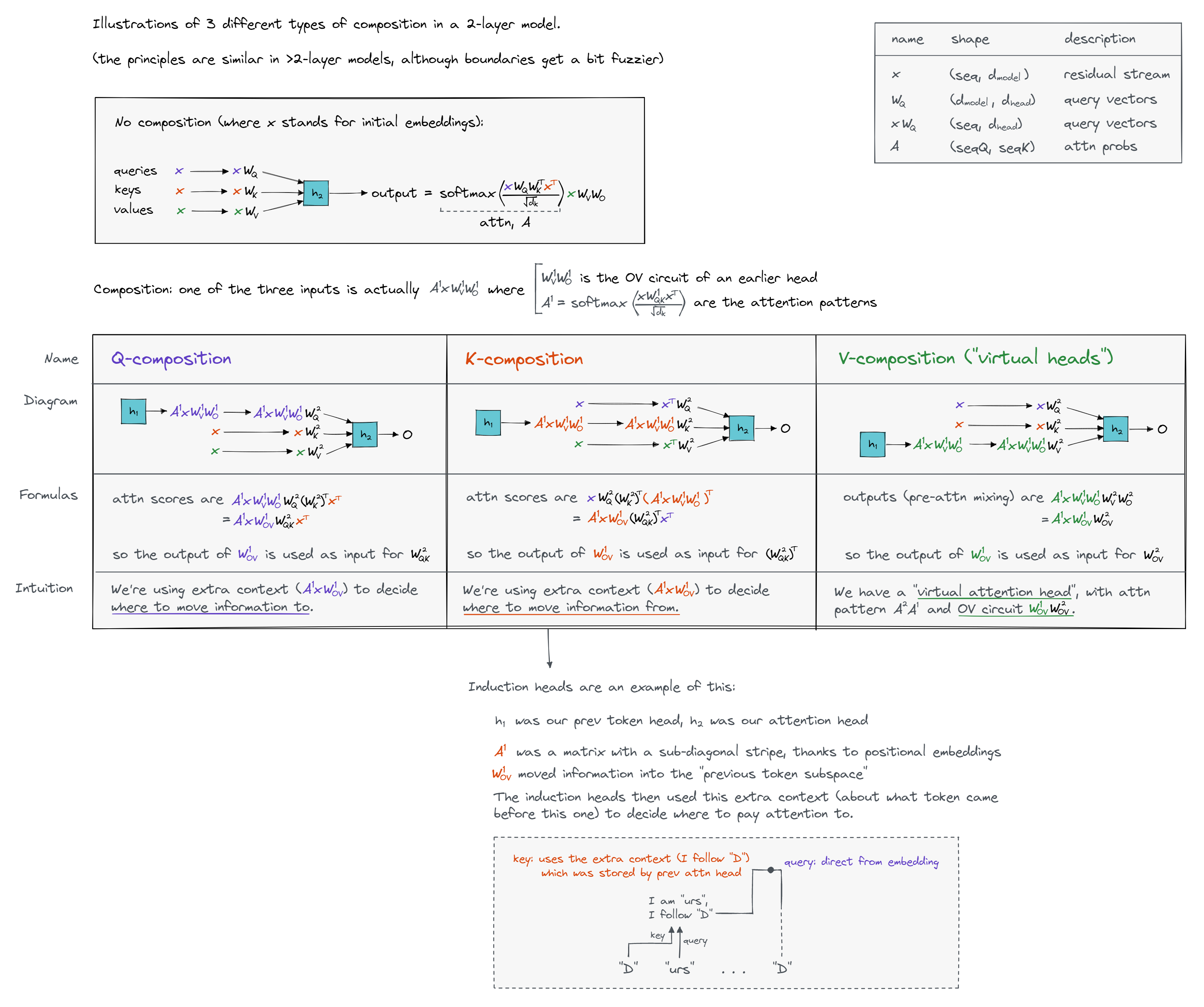
The key idea of compositional scores is that the residual stream is a large space, and each head is reading and writing from small subspaces. By default, any two heads will have little overlap between their subspaces (in the same way that any two random vectors have almost zero dot product in a large vector space). But if two heads are deliberately composing, then they will likely want to ensure they write and read from similar subspaces, so that minimal information is lost. As a result, we can just directly look at "how much overlap there is" between the output space of the earlier head and the K, Q, or V input space of the later head.
We represent the output space with $W_{OV}=W_V W_O$. Call matrices like this $W_A$.
We represent the input space with $W_{QK}=W_Q W_K^T$ (for Q-composition), $W_{QK}^T=W_K W_Q^T$ (for K-Composition) or $W_{OV}=W_V W_O$ (for V-Composition, of the later head). Call matrices like these $W_B$ (we've used this notation so that $W_B$ refers to a later head, and $W_A$ to an earlier head).
Help - I don't understand what motivates these definitions.
Recall that we can view each head as having three input wires (keys, queries and values), and one output wire (the outputs). The different forms of composition come from the fact that keys, queries and values can all be supplied from the output of a different head.
Here is an illustration which shows the three different cases, and should also explain why we use this terminology. You might have to open it in a new tab to see it clearly.
How do we formalise overlap? This is basically an open question, but a surprisingly good metric is $\frac{\|W_AW_B\|_F}{\|W_B\|_F\|W_A\|_F}$ where $\|W\|_F=\sqrt{\sum_{i,j}W_{i,j}^2}$ is the Frobenius norm, the square root of the sum of squared elements. (If you're dying of curiosity as to what makes this a good metric, you can jump to the section immediately after the exercises below.)
Exercise - calculate composition scores
Let's calculate this metric for all pairs of heads in layer 0 and layer 1 for each of K, Q and V composition and plot it.
We'll start by implementing this using plain old tensors (later on we'll see how this can be sped up using the FactoredMatrix class). We also won't worry about batching our calculations yet; we'll just do one matrix at a time.
We've given you tensors q_comp_scores etc. to hold the composition scores for each of Q, K and V composition (i.e. the [i, j]th element of q_comp_scores is the Q-composition score between the output from the ith head in layer 0 and the input to the jth head in layer 1). You should complete the function get_comp_score, and then fill in each of these tensors.
def get_comp_score(W_A: Float[Tensor, "in_A out_A"], W_B: Float[Tensor, "out_A out_B"]) -> float:
    """
    Return the composition score between W_A and W_B.
    """
    raise NotImplementedError()


tests.test_get_comp_score(get_comp_score)
Solution
def get_comp_score(W_A: Float[Tensor, "in_A out_A"], W_B: Float[Tensor, "out_A out_B"]) -> float:
    """
    Return the composition score between W_A and W_B.
    """
    W_A_norm = W_A.pow(2).sum().sqrt()
    W_B_norm = W_B.pow(2).sum().sqrt()
    W_AB_norm = (W_A @ W_B).pow(2).sum().sqrt()

    return (W_AB_norm / (W_A_norm * W_B_norm)).item()
Once you've passed the tests, you can fill in all the composition scores. Here you should just use a for loop, iterating over all possible pairs of W_A in layer 0 and W_B in layer 1, for each type of composition. Later on, we'll look at ways to batch this computation.
# Get all QK and OV matrices
W_QK = model.W_Q @ model.W_K.transpose(-1, -2)
W_OV = model.W_V @ model.W_O

# Define tensors to hold the composition scores
composition_scores = {
    "Q": t.zeros(model.cfg.n_heads, model.cfg.n_heads).to(device),
    "K": t.zeros(model.cfg.n_heads, model.cfg.n_heads).to(device),
    "V": t.zeros(model.cfg.n_heads, model.cfg.n_heads).to(device),
}

# YOUR CODE HERE - fill in values of the `composition_scores` dict, using `get_comp_score`

# Plot the composition scores
for comp_type in ["Q", "K", "V"]:
    plot_comp_scores(model, composition_scores[comp_type], f"{comp_type} Composition Scores")
Click to see the expected output
Solution
for i in tqdm(range(model.cfg.n_heads)):
    for j in range(model.cfg.n_heads):
        composition_scores["Q"][i, j] = get_comp_score(W_OV[0, i], W_QK[1, j])
        composition_scores["K"][i, j] = get_comp_score(W_OV[0, i], W_QK[1, j].T)
        composition_scores["V"][i, j] = get_comp_score(W_OV[0, i], W_OV[1, j])
Exercise - Setting a Baseline
To interpret the above graphs we need a baseline! A good one is what the scores look like at initialisation. Make a function that randomly generates a composition score 200 times and tries this. Remember to generate 4 [d_head, d_model] matrices, not 2 [d_model, d_model] matrices! This model was initialised with Kaiming Uniform Initialisation:
W = t.empty(shape)
nn.init.kaiming_uniform_(W, a=np.sqrt(5))
(Ideally we'd do a more efficient generation involving batching, and more samples, but we won't worry about that yet.)
def generate_single_random_comp_score() -> float:
    """
    Write a function which generates a single composition score for random matrices
    """
    raise NotImplementedError()


n_samples = 300
comp_scores_baseline = np.zeros(n_samples)
for i in tqdm(range(n_samples)):
    comp_scores_baseline[i] = generate_single_random_comp_score()

print("\nMean:", comp_scores_baseline.mean())
print("Std:", comp_scores_baseline.std())

hist(
    comp_scores_baseline,
    nbins=50,
    width=800,
    labels={"x": "Composition score"},
    title="Random composition scores",
)
Click to see the expected output
Solution
def generate_single_random_comp_score() -> float:
    """
    Write a function which generates a single composition score for random matrices
    """
    W_A_left = t.empty(model.cfg.d_model, model.cfg.d_head)
    W_B_left = t.empty(model.cfg.d_model, model.cfg.d_head)
    W_A_right = t.empty(model.cfg.d_model, model.cfg.d_head)
    W_B_right = t.empty(model.cfg.d_model, model.cfg.d_head)

    for W in [W_A_left, W_B_left, W_A_right, W_B_right]:
        nn.init.kaiming_uniform_(W, a=np.sqrt(5))

    W_A = W_A_left @ W_A_right.T
    W_B = W_B_left @ W_B_right.T

    return get_comp_score(W_A, W_B)
We can re-plot our above graphs with this baseline set to white. Look for interesting things in this graph!
baseline = comp_scores_baseline.mean()
for comp_type, comp_scores in composition_scores.items():
    plot_comp_scores(model, comp_scores, f"{comp_type} Composition Scores", baseline=baseline)
Click to see the expected output
Some interesting things to observe:
The most obvious thing that jumps out (when considered in the context of all the analysis we've done so far) is the K-composition scores. 0.7 (the prev token head) is strongly composing with 1.4 and 1.10 (the two attention heads). This is what we expect, and is a good indication that our composition scores are working as intended.
Another interesting thing to note is that the V-composition scores for heads 1.4 and 1.10 with all other heads in layer 0 are very low. In the context of the induction circuit, this is a good thing - the OV circuits of our induction heads should be operating on the embeddings, rather than the outputs of the layer-0 heads. (If our repeating sequence is A B ... A B, then it's the QK circuit's job to make sure the second A attends to the first B, and it's the OV circuit's job to project the residual vector at that position onto the embedding space in order to extract the B-information, while hopefully ignoring anything else that has been written to that position by the heads in layer 0). So once again, this is a good sign for our composition scores.
Theory + Efficient Implementation
So, what's up with that metric? The key is a cute linear algebra result that the squared Frobenius norm is equal to the sum of the squared singular values.
Proof
We'll give three different proofs:
Short sketch of proof
Clearly $\|M\|_F^2$ equals the sum of squared singular values when $M$ is diagonal. The singular values of $M$ don't change when we multiply it by an orthogonal matrix (only the matrices $U$ and $V$ will change, not $S$), so it remains to show that the Frobenius norm also won't change when we multiply $M$ by an orthogonal matrix. But this follows from the fact that the Frobenius norm is the sum of the squared $l_2$ norms of the column vectors of $M$, and orthogonal matrices preserve $l_2$ norms. (If we're right-multiplying $M$ by an orthogonal matrix, then we instead view this as performing orthogonal operations on the row vectors of $M$, and the same argument holds.)
Long proof
Each of the terms in large brackets is actually the dot product of columns of $U$ and $V$ respectively. Since these are orthogonal matrices, these terms evaluate to 1 when $k_1=k_2$ and 0 otherwise. So we are left with:
Cute proof which uses the fact that the squared Frobenius norm $|M|^2$ is the same as the trace of $MM^T$
where we used the cyclicity of trace, and the fact that $U$ is orthogonal so $U^TU=I$ (and same for $V$). We finish by observing that $\|S\|_F^2$ is precisely the sum of the squared singular values.
So if $W_A=U_AS_AV_A^T$, $W_B=U_BS_BV_B^T$, then $\|W_A\|_F=\|S_A\|_F$, $\|W_B\|_F=\|S_B\|_F$ and $\|W_AW_B\|_F=\|S_AV_A^TU_BS_B\|_F$. In some sense, $V_A^TU_B$ represents how aligned the subspaces written to and read from are, and the $S_A$ and $S_B$ terms weights by the importance of those subspaces.
Click here, if this explanation still seems confusing.
$U_B$ is a matrix of shape [d_model, d_head]. It represents the subspace being read from, i.e. our later head reads from the residual stream by projecting it onto the d_head columns of this matrix.
$V_A$ is a matrix of shape [d_model, d_head]. It represents the subspace being written to, i.e. the thing written to the residual stream by our earlier head is a linear combination of the d_head column-vectors of $V_A$.
$V_A^T U_B$ is a matrix of shape [d_head, d_head]. Each element of this matrix is formed by taking the dot product of two vectors of length d_model:
- $v_i^A$, a column of $V_A$ (one of the vectors our earlier head embeds into the residual stream)
- $u_j^B$, a column of $U_B$ (one of the vectors our later head projects the residual stream onto)
Let the singular values of $S_A$ be $\sigma_1^A, ..., \sigma_k^A$ and similarly for $S_B$. Then:
This is a weighted sum of the squared cosine similarity of the columns of $V_A$ and $U_B$ (i.e. the output directions of the earlier head and the input directions of the later head). The weights in this sum are given by the singular values of both $S_A$ and $S_B$ - i.e. if $v^A_i$ is an important output direction, and $u_B^i$ is an important input direction, then the composition score will be much higher when these two directions are aligned with each other.
To build intuition, let's consider a couple of extreme examples.
- If there was no overlap between the spaces being written to and read from, then $V_A^T U_B$ would be a matrix of zeros (since every $v_i^A \cdot u_j^B$ would be zero). This would mean that the composition score would be zero.
- If there was perfect overlap, i.e. the span of the $v_i^A$ vectors and $u_j^B$ vectors is the same, then the composition score is large. It is as large as possible when the most important input directions and most important output directions line up (i.e. when the singular values $\sigma_i^A$ and $\sigma_j^B$ are in the same order).
- If our matrices $W_A$ and $W_B$ were just rank 1 (i.e. $W_A = \sigma_A u_A v_A^T$, and $W_B = \sigma_B u_B v_B^T$), then the composition score is $|v_A^T u_B|$, in other words just the cosine similarity of the single output direction of $W_A$ and the single input direction of $W_B$.
Exercise - batching, and using the FactoredMatrix class
We can also use this insight to write a more efficient way to calculate composition scores - this is extremely useful if you want to do this analysis at scale! The key is that we know that our matrices have a low rank factorisation, and it's much cheaper to calculate the SVD of a narrow matrix than one that's large in both dimensions. See the algorithm described at the end of the paper (search for SVD).
So we can work with the FactoredMatrix class. This also provides the method .norm() which returns the Frobenium norm. This is also a good opportunity to bring back batching - this will sometimes be useful in our analysis. In the function below, W_As and W_Bs are both >2D factored matrices (e.g. they might represent the OV circuits for all heads in a particular layer, or across multiple layers), and the function's output should be a tensor of composition scores for each pair of matrices (W_A, W_B) in the >2D tensors (W_As, W_Bs).
def get_batched_comp_scores(W_As: FactoredMatrix, W_Bs: FactoredMatrix) -> Tensor:
    """
    Computes the compositional scores from indexed factored matrices W_As and W_Bs.

    Each of W_As and W_Bs is a FactoredMatrix object which is indexed by all but its last 2
    dimensions, i.e.:
        W_As.shape == (*A_idx, A_in, A_out)
        W_Bs.shape == (*B_idx, B_in, B_out)
        A_out == B_in

    Return: tensor of shape (*A_idx, *B_idx) where the [*a_idx, *b_idx]th element is the
    compositional score from W_As[*a_idx] to W_Bs[*b_idx].
    """
    raise NotImplementedError()


W_QK = FactoredMatrix(model.W_Q, model.W_K.transpose(-1, -2))
W_OV = FactoredMatrix(model.W_V, model.W_O)

composition_scores_batched = dict()
composition_scores_batched["Q"] = get_batched_comp_scores(W_OV[0], W_QK[1])
composition_scores_batched["K"] = get_batched_comp_scores(
    W_OV[0], W_QK[1].T
)  # Factored matrix: .T is interpreted as transpose of the last two axes
composition_scores_batched["V"] = get_batched_comp_scores(W_OV[0], W_OV[1])

t.testing.assert_close(composition_scores_batched["Q"], composition_scores["Q"])
t.testing.assert_close(composition_scores_batched["K"], composition_scores["K"])
t.testing.assert_close(composition_scores_batched["V"], composition_scores["V"])
print("Tests passed - your `get_batched_comp_scores` function is working!")
Hint
Suppose W_As has shape (A1, A2, ..., Am, A_in, A_out) and W_Bs has shape (B1, B2, ..., Bn, B_in, B_out) (where A_out == B_in).
It will be helpful to reshape these two tensors so that:
W_As.shape == (A1*A2*...*Am, 1, A_in, A_out)
W_Bs.shape == (1, B1*B2*...*Bn, B_in, B_out)
since we can then multiply them together as W_As @ W_Bs (broadcasting will take care of this for us!).
To do the reshaping, the easiest way is to reshape W_As.A and W_As.B, and define a new FactoredMatrix from these reshaped tensors (and same for W_Bs).
Solution
def get_batched_comp_scores(W_As: FactoredMatrix, W_Bs: FactoredMatrix) -> Tensor:
    """
    Computes the compositional scores from indexed factored matrices W_As and W_Bs.

    Each of W_As and W_Bs is a FactoredMatrix object which is indexed by all but its last 2
    dimensions, i.e.:
        W_As.shape == (*A_idx, A_in, A_out)
        W_Bs.shape == (*B_idx, B_in, B_out)
        A_out == B_in

    Return: tensor of shape (*A_idx, *B_idx) where the [*a_idx, *b_idx]th element is the
    compositional score from W_As[*a_idx] to W_Bs[*b_idx].
    """
    # Flatten W_As into (single_A_idx, 1, A_in, A_out)
    W_As = FactoredMatrix(
        W_As.A.reshape(-1, 1, *W_As.A.shape[-2:]),
        W_As.B.reshape(-1, 1, *W_As.B.shape[-2:]),
    )
    # Flatten W_Bs into (1, single_B_idx, B_in(=A_out), B_out)
    W_Bs = FactoredMatrix(
        W_Bs.A.reshape(1, -1, *W_Bs.A.shape[-2:]),
        W_Bs.B.reshape(1, -1, *W_Bs.B.shape[-2:]),
    )

    # Compute the product, with shape (single_A_idx, single_B_idx, A_in, B_out)
    W_ABs = W_As @ W_Bs

    # Compute the norms, and return the metric
    return W_ABs.norm() / (W_As.norm() * W_Bs.norm())
Targeted Ablations
We can refine the ablation technique to detect composition by looking at the effect of the ablation on the attention pattern of an induction head, rather than the loss. Let's implement this!
Gotcha - by default, run_with_hooks removes any existing hooks when it runs. If you want to use caching, set the reset_hooks_start flag to False.
seq_len = 50


def ablation_induction_score(prev_head_index: int | None, ind_head_index: int) -> float:
    """
    Takes as input the index of the L0 head and the index of the L1 head, and then runs with the
    previous token head ablated and returns the induction score for the ind_head_index now.
    """

    def ablation_hook(v, hook):
        if prev_head_index is not None:
            v[:, :, prev_head_index] = 0.0
        return v

    def induction_pattern_hook(attn, hook):
        hook.ctx[prev_head_index] = attn[0, ind_head_index].diag(-(seq_len - 1)).mean()

    model.run_with_hooks(
        rep_tokens,
        fwd_hooks=[
            (utils.get_act_name("v", 0), ablation_hook),
            (utils.get_act_name("pattern", 1), induction_pattern_hook),
        ],
    )
    return model.blocks[1].attn.hook_pattern.ctx[prev_head_index].item()


baseline_induction_score = ablation_induction_score(None, 4)
print(f"Induction score for no ablations: {baseline_induction_score:.5f}\n")
for i in range(model.cfg.n_heads):
    new_induction_score = ablation_induction_score(i, 4)
    induction_score_change = new_induction_score - baseline_induction_score
    print(f"Ablation score change for head {i:02}: {induction_score_change:+.5f}")
Question - what is the interpretation of the results you're getting?
You should have found that the induction score without any ablations is about 0.68, and that most other heads don't change the induction score by much when they are ablated, except for head 7 which reduces the induction score to nearly zero.
This is another strong piece of evidence that head 0.7 is the prev token head in this induction circuit.
Bonus
Looking for Circuits in Real LLMs
A particularly cool application of these techniques is looking for real examples of circuits in large language models. Fortunately, there's a bunch of open source ones you can play around with in the TransformerLens library! Many of the techniques we've been using for our 2L transformer carry over to ones with more layers.
This library should make it moderately easy to play around with these models - I recommend going wild and looking for interesting circuits!
Some fun things you might want to try:
- Look for induction heads - try repeating all of the steps from above. Do they follow the same algorithm?
- Look for neurons that erase info
- i.e. having a high negative cosine similarity between the input and output weights
- Try to interpret a position embedding.
Positional Embedding Hint
Look at the singular value decomposition t.svd and plot the principal components over position space. High ones tend to be sine and cosine waves of different frequencies.
- Look for heads with interpretable attention patterns: e.g. heads that attend to the same word (or subsequent word) when given text in different languages, or the most recent proper noun, or the most recent full-stop, or the subject of the sentence, etc.
- Pick a head, ablate it, and run the model on a load of text with and without the head. Look for tokens with the largest difference in loss, and try to interpret what the head is doing.
- Try replicating some of Kevin's work on indirect object identification.
- Inspired by the ROME paper, use the causal tracing technique of patching in the residual stream - can you analyse how the network answers different facts?
Note: I apply several simplifications to the resulting transformer - these leave the model mathematically equivalent and doesn't change the output log probs, but does somewhat change the structure of the model and one change translates the output logits by a constant.
Model simplifications
Centering $W_U$
The output of $W_U$ is a $d_{vocab}$ vector (or tensor with that as the final dimension) which is fed into a softmax
LayerNorm Folding
LayerNorm is only applied at the start of a linear layer reading from the residual stream (eg query, key, value, mlp_in or unembed calculations)
Each LayerNorm has the functional form $LN:\mathbb{R}^n\to\mathbb{R}^n$, $LN(x)=s(x) * w_{ln} + b_{ln}$, where $*$ is element-wise multiply and $s(x)=\frac{x-\bar{x}}{|x-\bar{x}|}$, and $w_{ln},b_{ln}$ are both vectors in $\mathbb{R}^n$
The linear layer has form $l:\mathbb{R}^n\to\mathbb{R}^m$, $l(y)=Wy+b$ where $W\in \mathbb{R}^{m\times n},b\in \mathbb{R}^m,y\in\mathbb{R}^n$
So $f(LN(x))=W(w_{ln} * s(x)+b_{ln})+b=(W * w_{ln})s(x)+(Wb_{ln}+b)=W_{eff}s(x)+b_{eff}$, where $W_{eff}$ is the elementwise product of $W$ and $w_{ln}$ (showing that elementwise multiplication commutes like this is left as an exercise) and $b_{eff}=Wb_{ln}+b\in \mathbb{R}^m$.
From the perspective of interpretability, it's much nicer to interpret the folded layer $W_{eff},b_{eff}$ - fundamentally, this is the computation being done, and there's no reason to expect $W$ or $w_{ln}$ to be meaningful on their own.
Training Your Own Toy Models
A fun exercise is training models on the minimal task that'll produce induction heads - predicting the next token in a sequence of random tokens with repeated subsequences. You can get a small 2L Attention-Only model to do this.
Tips
- Make sure to randomise the positions that are repeated! Otherwise the model can just learn the boring algorithm of attending to fixed positions
- It works better if you only evaluate loss on the repeated tokens, this makes the task less noisy.
- It works best with several repeats of the same sequence rather than just one.
- If you do things right, and give it finite data + weight decay, you should be able to get it to grok - this may take some hyper-parameter tuning though.
- When I've done this I get weird franken-induction heads, where each head has 1/3 of an induction stripe, and together cover all tokens.
- It'll work better if you only let the queries and keys access the positional embeddings, but should work either way.
Interpreting Induction Heads During Training
A particularly striking result about induction heads is that they consistently form very abruptly in training as a phase change, and are such an important capability that there is a visible non-convex bump in the loss curve (in this model, approx 2B to 4B tokens). I have a bunch of checkpoints for this model, you can try re-running the induction head detection techniques on intermediate checkpoints and see what happens. (Bonus points if you have good ideas for how to efficiently send a bunch of 300MB checkpoints from Wandb lol)
Further discussion / investigation
Anthropic has written a post on In-context Learning and Induction Heads which goes into much deeper discussion on induction heads. The post is structured around six different points of evidence for the hypothesis that induction heads are the main source of in-context learning in transformer models, even large ones. Briefly, these are:
- Transformers undergo a "phase change" where they suddenly become much better at in-context learning, and this is around the same time induction heads appear.
- When we change the transformer's architecture to make it easier for induction heads to form, we get a corresponding improvement in in-context learning.
- When we ablate induction heads at runtime, in-context learning gets worse.
- We have specific examples of induction heads performing more complex in-context learning algorithms (you'll have the opportunity to investigate one of these later - indirect object identification).
- We have a mechanistic explanation of induction heads, which suggests natural extensions to more general forms of in-context learning.
- In-context learning-related behaviour is generally smoothly continuous between small and large models, suggesting that the underlying mechanism is also the same.
Here are a few questions for you:
- How compelling do you find this evidence? Discuss with your partner.
- Which points do you find most compelling?
- Which do you find least compelling?
- Are there any subset of these which would be enough to convince you of the hypothesis, in the absence of others?
- In point 3, the paper observes that in-context learning performance degrades when you ablate induction heads. While we measured this by testing the model's ability to copy a duplicated random sequence, the paper used in-context learning score (the loss of the 500th token in the context, minus the loss on the 50th token).
- Can you see why this is a reasonable metric?
- Can you replicate these results (maybe on a larger model than the 2-layer one we've been using)?
- In point 4 (more complex forms of in-context learning), the paper suggests the natural extension of "fuzzy induction heads", which match patterns like
[A*][B*]...[A][B]rather than[A][B]...[A][B](where the*indicates some form of linguistic similarity, not necessarily being the same token).- Can you think of any forms this might take, i.e. any kinds of similarity which induction heads might pick up on? Can you generate examples?