2️⃣ Clean Transformer Implementation
Learning Objectives
- Understand that a transformer is composed of attention heads and MLPs, with each one performing operations on the residual stream
- Understand that the attention heads in a single layer operate independently, and that they have the role of calculating attention patterns (which determine where information is moved to & from in the residual stream)
- Learn about & implement the following transformer modules:
- LayerNorm (transforming the input to have zero mean and unit variance)
- Positional embedding (a lookup table from position indices to residual stream vectors)
- Attention (the method of computing attention patterns for residual stream vectors)
- MLP (the collection of linear and nonlinear transformations which operate on each residual stream vector in the same way)
- Embedding (a lookup table from tokens to residual stream vectors)
- Unembedding (a matrix for converting residual stream vectors into a distribution over tokens)
High-Level architecture
Go watch Neel's Transformer Circuits walkthrough if you want more intuitions!
(Diagram is bottom to top, right-click and open for higher resolution.)
![]()
Tokenization & Embedding
The input tokens $t$ are integers. We get them from taking a sequence, and tokenizing it (like we saw in the previous section).
The token embedding is a lookup table mapping tokens to vectors, which is implemented as a matrix $W_E$. The matrix consists of a stack of token embedding vectors (one for each token).
Residual stream
The residual stream is the sum of all previous outputs of layers of the model, and is also the input to each new layer. It has shape [batch, seq_len, d_model] (where d_model is the length of a single embedding vector).
The initial value of the residual stream is denoted $x_0$ in the diagram, and $x_i$ are later values of the residual stream (after more attention and MLP layers have been applied to the residual stream).
The residual stream is really fundamental. It's the central object of the transformer. It's how model remembers things, moves information between layers for composition, and it's the medium used to store the information that attention moves between positions.
Aside - logit lens
A key idea of transformers is the [residual stream as output accumulation](https://www.lesswrong.com/posts/X26ksz4p3wSyycKNB/gears-level-mental-models-of-transformer-interpretability#Residual_Stream_as_Output_Accumulation:~:text=The%20Models-,Residual%20Stream%20as%20Output%20Accumulation,-The%20residual%20stream). As we move through the layers of the model, shifting information around and processing it, the values in the residual stream represent the accumulation of all the inferences made by the transformer up to that point.
This is neatly illustrated by the logit lens. Rather than getting predictions from the residual stream at the very end of the model, we can take the value of the residual stream midway through the model and convert it to a distribution over tokens. When we do this, we find surprisingly coherent predictions, especially in the last few layers before the end.
Transformer blocks
Then we have a series of n_layers transformer blocks (also sometimes called residual blocks).
Note - a block contains an attention layer and an MLP layer, but we say a transformer has $k$ layers if it has $k$ blocks (i.e. $2k$ total layers).
![]()
Attention
First we have attention. This moves information from prior positions in the sequence to the current token.
We do this for every token in parallel using the same parameters. The only difference is that we look backwards only (to avoid "cheating"). This means later tokens have more of the sequence that they can look at.
Attention layers are the only bit of a transformer that moves information between positions (i.e. between vectors at different sequence positions in the residual stream).
Attention layers are made up of n_heads heads - each with their own parameters, own attention pattern, and own information how to copy things from source to destination. The heads act independently and additively, we just add their outputs together, and back to the stream.
Each head does the following: * Produces an attention pattern for each destination token, a probability distribution of prior source tokens (including the current one) weighting how much information to copy. * Moves information (via a linear map) in the same way from each source token to each destination token.
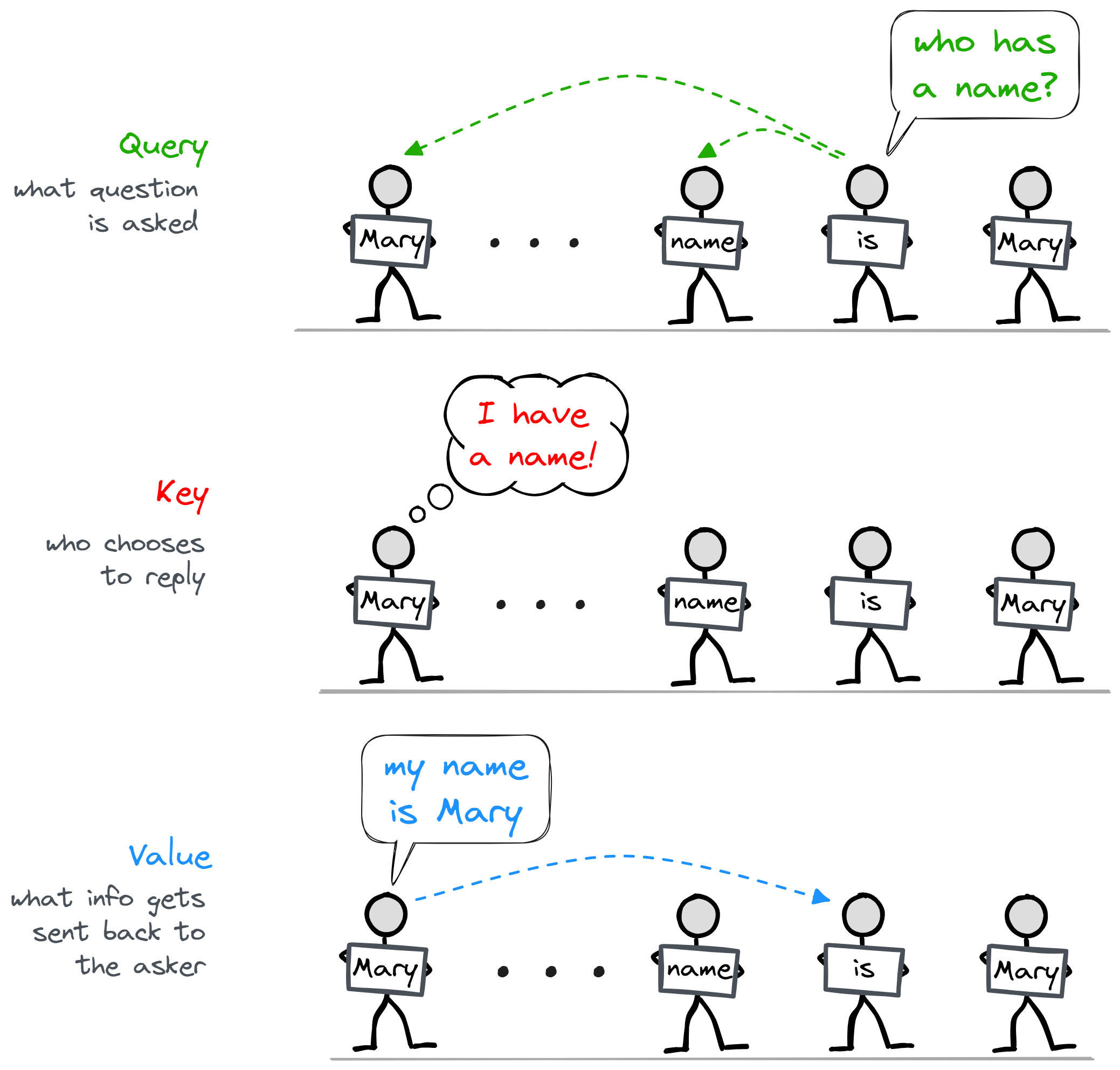
Each attention head is made up of three components: the keys, queries, and values (often abbreviated as K, Q and V). These names come from their analogy to retrieval systems. Broadly speaking:
- Queries represent a question or request for information, e.g. "I'm looking for a name that appeared earlier in this sentence".
- Keys represent whether a source token's information matches the query, e.g. if the source token is "Mary" then this causes the key to have a high dot product with the query (we call this an attention score), and it means that a lot of information will be taken from this token.
- Values represent the information that actually gets moved. This sounds similar to keys, but it's actually different in an important way. For instance, the key might just contain the information "this is a name", but the value could be the actual name itself.
The diagram below illustrates the three different parts, in the context of the analogy for transformers we introduced earlier. This is a simplified model for how the person holding the "in" token might come to figure out that the next token is "Mary". In later sections we'll look at the actual function performed by attention heads and see how the operations relate to this analogy.
Another interesting intuition for attention is as a kind of "generalized convolution" - read the dropdown below if you want to learn more about this.
Intuition - attention as generalized convolution
We can think of attention as a kind of generalized convolution. Standard convolution layers work by imposing a "prior of locality", i.e. the assumption that pixels which are close together are more likely to share information. Although language has some locality (two words next to each other are more likely to share information than two words 100 tokens apart), the picture is a lot more nuanced, because which tokens are relevant to which others depends on the context of the sentence. For instance, in the sentence "When Mary and John went to the store, John gave a drink to Mary", the names in this sentence are the most important tokens for predicting that the final token will be "Mary", and this is because of the particular context of this sentence rather than the tokens' position.
Attention layers are effectively our way of saying to the transformer, "don't impose a prior of locality, but instead develop your own algorithm to figure out which tokens are important to which other tokens in any given sequence."
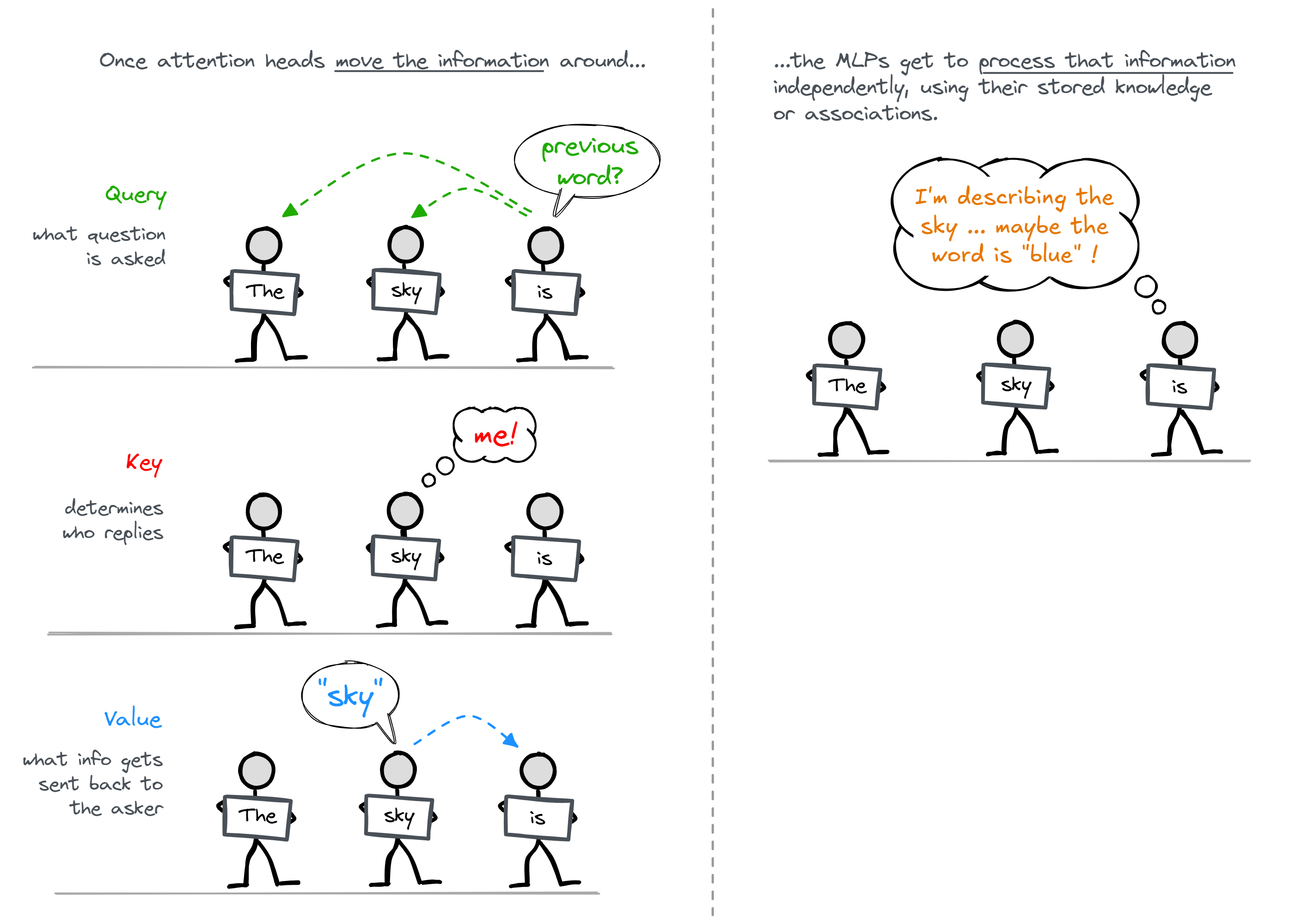
Below is a schematic diagram of the attention layers. We'll go into much more detail during the actual implementation, so don't worry if this doesn't fully make sense yet.
![]()
MLP
The MLP layers are just a standard neural network, with a singular hidden layer and a nonlinear activation function. The exact activation isn't conceptually important (GELU seems to perform best).
Our hidden dimension is normally d_mlp = 4 * d_model. Exactly why the ratios are what they are isn't super important (people basically cargo-cult what GPT did back in the day!).
Importantly, the MLP operates on positions in the residual stream independently, and in exactly the same way. It doesn't move information between positions.
Once attention has moved relevant information to a single position in the residual stream, MLPs can actually do computation, reasoning, lookup information, etc. What the hell is going on inside MLPs is a pretty big open problem in transformer mechanistic interpretability - see the Toy Model of Superposition Paper for more on why this is hard.
To go back to our analogy for transformers, we can essentially view MLPs as the thinking that each person in the line does once they've grabbed the information they need from the people behind them (via attention). Usually the MLP layers make up a much larger fraction of the model's total parameter count than attention layers (often around 2/3 although this varies between architectures), which makes sense since processing the information is a bigger task than just moving it around.
Here are a few more intuitions for MLPs, which you might find interesting:
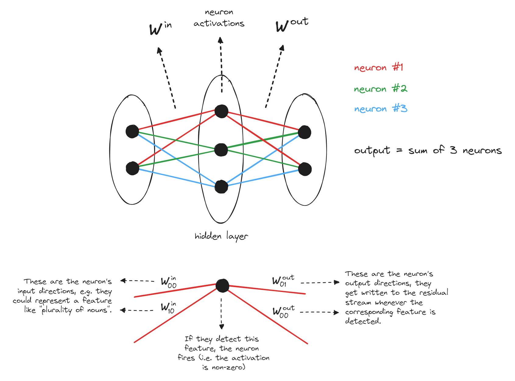
Intuition - MLPs as key-value pairs
We can write the MLP's output as $f(x^T W^{in})W^{out}$, where $W^{in}$ and $W^{out}$ are the different weights of the MLP (ignoring biases), $f$ is the activation function, and $x$ is a vector in the residual stream. This can be rewritten as:
We can view the vectors $W^{in}_{[:, i]}$ as the input directions, and $W^{out}_{[i, :]}$ as the output directions. We say the input directions are activated by certain textual features, and when they are activated, vectors are written in the corresponding output direction. This is very similar to the concept of keys and values in attention layers, which is why these vectors are also sometimes called keys and values (e.g. see the paper [Transformer Feed-Forward Layers Are Key-Value Memories](https://arxiv.org/pdf/2012.14913.pdf)).
Terminology note - sometimes we refer to each of these $d_{mlp}$ input-output pairs as neurons.
---
Here's a step-by-step breakdown of the linear algebra, if it was too fast above. We have:
where $W^{in}_{[:, i]}$ are the columns of $W^{in}$. In other words, these values (the pre-GELU activations) are projections of $x$ along the input directions of the neurons.
If we add our activation function and the second matrix, then we get:
where $W^{out}_{[i, :]}$ are the rows of $W^{out}$. In other words, our output is a linear combination of the rows of $W^{out}$, with the coefficients of that linear combination given by the projections of $x$ along the columns of $W^{in}$.
Intuition - MLPs as knowledge storage
We can think of MLPs as where knowledge gets stored in our transformer. The attention mechanism is what moves information around between sequence positions, but the MLPs is where this information is processed, and new information is written into the residual stream which is a function of the old information.
This is deeply connected to the key-value pairs model, since you can treat key-value pairs as a kind of associative memory system (where the key serves as a unique identifier, and the value holds the related information).
Another related intuition (for which there is some evidence) is MLPs as memory management. In an idealized case, we might find that the $i$-th neuron satisfies $W^{in}_{[:, i]} \approx - W^{out}_{[i, :]} \approx \vec v$ for some unit vector $\vec v$, meaning it may be responsible for erasing the positive component of vector $\vec x$ in the direction $\vec v$ (exercise - can you show why this is the case?). This can free up space in the residual stream for other components to write to.
Lastly, here's a schematic diagram of the MLP layers. Again, we'll go into much more detail during the actual implementation, so don't worry if this doesn't fully make sense yet.
![]()
Unembedding
Finally, we unembed!
This just consists of applying a linear map $W_U$, going from final residual stream to a vector of logits - this is the output.
Aside - tied embeddings
Note - sometimes we use something called a tied embedding - this is where we use the same weights for our $W_E$ and $W_U$ matrices. In other words, to get the logit score for a particular token at some sequence position, we just take the vector in the residual stream at that sequence position and take the inner product with the corresponding token embedding vector. This is more training-efficient (because there are fewer parameters in our model), and it might seem principled at first. After all, if two words have very similar meanings, shouldn't they have similar embedding vectors because the model will treat them the same, and similar unembedding vectors because they could both be substituted for each other in most output?
However, this is actually not very principled, for the following main reason: the direct path involving the embedding and unembedding should approximate bigram frequencies.
Let's break down this claim. Bigram frequencies refers to the frequencies of pairs of words in the english language (e.g. the bigram frequency of "Barack Obama" is much higher than the product of the individual frequencies of the words "Barack" and "Obama"). If our model had no attention heads or MLP layers, then all we have is a linear map from our one-hot encoded token T to a probability distribution over the token following T. This map is represented by the linear transformation $t \to t^T W_E W_U$ (where $t$ is our one-hot encoded token vector). Since the output of this transformation can only be a function of the token T (and no earlier tokens), the best we can do is have this map approximate the true frequency of bigrams starting with T, which appear in the training data. Importantly, this is not a symmetric map. We want T = "Barack" to result in a high probability of the next token being "Obama", but not the other way around!
Even in multi-layer models, a similar principle applies. There will be more paths through the model than just the "direct path" $W_E W_U$, but because of the residual connections there will always exist a direct path, so there will always be some incentive for $W_E W_U$ to approximate bigram frequencies.
That being said, smaller (<8B parameter) LLMs still often use tied embeddings to improve training and inference efficiency. It can be easier to start from tied weights and then use MLP0 to break the symmetry than to initialize encoder and decoder with no shared structure at all.
Bonus things - less conceptually important but key technical details
LayerNorm
- Simple normalization function applied at the start of each layer (i.e. before each MLP, attention layer, and before the unembedding)
- Converts each input vector (independently in parallel for each
(batch, seq)residual stream vector) to have mean zero and variance 1. - Then applies an elementwise scaling and translation
- Cool maths tangent: The scale ($\odot \gamma$) & translate ($+ \beta$) is just a linear map. LayerNorm is only applied immediately before another linear map (either the MLP, or the query/key/value linear maps in the attention head, or the unembedding $W_U$). Linear compose linear = linear, so we can just fold this into a single effective linear layer and ignore it.
fold_ln=Trueflag infrom_pretraineddoes this for you.
- LayerNorm is annoying for interpretability - it would be linear if not for the fact we divide by the variance, so you can't decompose the contributions of the input to the output independently. But it's almost linear - if you're changing a small part of the input you can pretend $\sqrt{\text{Var}[x] + \epsilon}$ is constant, so the LayerNorm operation is linear, but if you're changing $x$ enough to alter the norm substantially it's not linear.
![]()
Positional embeddings
- Problem: Attention operates over all pairs of positions. This means it's symmetric with regards to position - the attention calculation from token 5 to token 1 and token 5 to token 2 are the same by default
- This is dumb because nearby tokens are more relevant.
- There's a lot of dumb hacks for this.
- We'll focus on learned, absolute positional embeddings. This means we learn a lookup table mapping the index of the position of each token to a residual stream vector, and add this to the embed.
- Note that we add rather than concatenate. This is because the residual stream is shared memory, and likely under significant superposition (the model compresses more features in there than the model has dimensions)
- We basically never concatenate inside a transformer, unless doing weird shit like generating text efficiently.
- This connects to attention as generalized convolution
- We argued that language does still have locality, and so it's helpful for transformers to have access to the positional information so they "know" two tokens are next to each other (and hence probably relevant to each other).
Actual Code!
Model architecture table (this will be helpful for understanding the results you get when running the code block below):
| Parameter | Value |
|---|---|
| batch | 1 |
| position | 35 |
| d_model | 768 |
| n_heads | 12 |
| n_layers | 12 |
| d_mlp | 3072 (= 4 * d_model) |
| d_head | 64 (= d_model / n_heads) |
Parameters and Activations
It's important to distinguish between parameters and activations in the model.
- Parameters are the weights and biases that are learned during training.
- These don't change when the model input changes.
- Activations are temporary numbers calculated during a forward pass, that are functions of the input.
- We can think of these values as only existing for the duration of a single forward pass, and disappearing afterwards.
- We can use hooks to access these values during a forward pass (more on hooks later), but it doesn't make sense to talk about a model's activations outside the context of some particular input.
- Attention scores and patterns are activations (this is slightly non-intuitve because they're used in a matrix multiplication with another activation).
Print All Activation Shapes of Reference Model
Run the following code to print all the activation shapes of the reference model:
for activation_name, activation in cache.items():
    # Only print for first layer
    if ".0." in activation_name or "blocks" not in activation_name:
        print(f"{activation_name:30} {tuple(activation.shape)}")
hook_embed                     (1, 35, 768)
hook_pos_embed                 (1, 35, 768)
blocks.0.hook_resid_pre        (1, 35, 768)
blocks.0.ln1.hook_scale        (1, 35, 1)
blocks.0.ln1.hook_normalized   (1, 35, 768)
blocks.0.attn.hook_q           (1, 35, 12, 64)
blocks.0.attn.hook_k           (1, 35, 12, 64)
blocks.0.attn.hook_v           (1, 35, 12, 64)
blocks.0.attn.hook_attn_scores (1, 12, 35, 35)
blocks.0.attn.hook_pattern     (1, 12, 35, 35)
blocks.0.attn.hook_z           (1, 35, 12, 64)
blocks.0.hook_attn_out         (1, 35, 768)
blocks.0.hook_resid_mid        (1, 35, 768)
blocks.0.ln2.hook_scale        (1, 35, 1)
blocks.0.ln2.hook_normalized   (1, 35, 768)
blocks.0.mlp.hook_pre          (1, 35, 3072)
blocks.0.mlp.hook_post         (1, 35, 3072)
blocks.0.hook_mlp_out          (1, 35, 768)
blocks.0.hook_resid_post       (1, 35, 768)
ln_final.hook_scale            (1, 35, 1)
ln_final.hook_normalized       (1, 35, 768)
Print All Parameters Shapes of Reference Model
for name, param in reference_gpt2.named_parameters():
    # Only print for first layer
    if ".0." in name or "blocks" not in name:
        print(f"{name:18} {tuple(param.shape)}")
embed.W_E          (50257, 768)
pos_embed.W_pos    (1024, 768)
blocks.0.ln1.w     (768,)
blocks.0.ln1.b     (768,)
blocks.0.ln2.w     (768,)
blocks.0.ln2.b     (768,)
blocks.0.attn.W_Q  (12, 768, 64)
blocks.0.attn.W_O  (12, 64, 768)
blocks.0.attn.b_Q  (12, 64)
blocks.0.attn.b_O  (768,)
blocks.0.attn.W_K  (12, 768, 64)
blocks.0.attn.W_V  (12, 768, 64)
blocks.0.attn.b_K  (12, 64)
blocks.0.attn.b_V  (12, 64)
blocks.0.mlp.W_in  (768, 3072)
blocks.0.mlp.b_in  (3072,)
blocks.0.mlp.W_out (3072, 768)
blocks.0.mlp.b_out (768,)
ln_final.w         (768,)
ln_final.b         (768,)
unembed.W_U        (768, 50257)
unembed.b_U        (50257,)
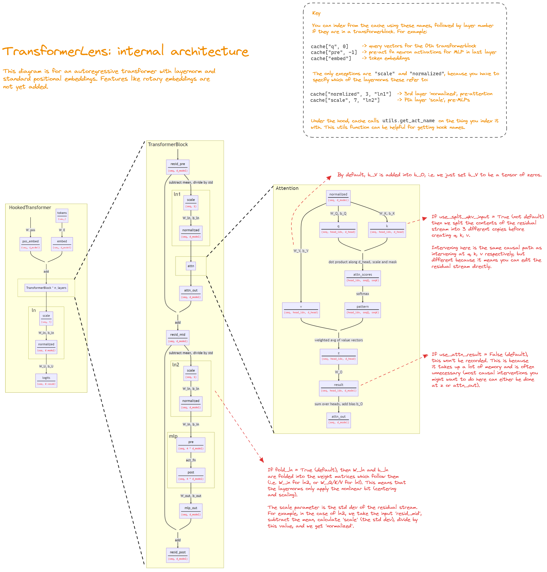
This diagram shows the name of all activations and parameters in a fully general transformer model from transformerlens (except for a few at the start and end, like the embedding and unembedding). Lots of this won't make sense at first, but you can return to this diagram later and check that you understand most/all parts of it.
There's also an annotated version here.
Config
The config object contains all the hyperparameters of the model. We can print the config of the reference model to see what it contains:
# As a reference - note there's a lot of stuff we don't care about in here, to do with library internals or other architectures
print(reference_gpt2.cfg)
HookedTransformerConfig:
{'act_fn': 'gelu_new',
 'attention_dir': 'causal',
 'attn_only': False,
 'attn_scale': 8.0,
 'attn_scores_soft_cap': -1.0,
 'attn_types': None,
 'checkpoint_index': None,
 'checkpoint_label_type': None,
 'checkpoint_value': None,
 'd_head': 64,
 'd_mlp': 3072,
 'd_model': 768,
 'd_vocab': 50257,
 ...
 'use_split_qkv_input': False,
 'window_size': None}
We define a stripped down config for our model:
@dataclass
class Config:
    d_model: int = 768
    debug: bool = True
    layer_norm_eps: float = 1e-5
    d_vocab: int = 50257
    init_range: float = 0.02
    n_ctx: int = 1024
    d_head: int = 64
    d_mlp: int = 3072
    n_heads: int = 12
    n_layers: int = 12


cfg = Config()
print(cfg)
Config(d_model=768, debug=True, layer_norm_eps=1e-05, d_vocab=50257, init_range=0.02, n_ctx=1024, d_head=64, d_mlp=3072, n_heads=12, n_layers=12)
Tests
Tests are great, write lightweight ones to use as you go!
Naive test: Generate random inputs of the right shape, input to your model, check whether there's an error and print the correct output.
def rand_float_test(cls, shape):
    cfg = Config(debug=True)
    layer = cls(cfg).to(device)
    random_input = t.randn(shape).to(device)
    print("Input shape:", random_input.shape)
    output = layer(random_input)
    if isinstance(output, tuple):
        output = output[0]
    print("Output shape:", output.shape, "\n")


def rand_int_test(cls, shape):
    cfg = Config(debug=True)
    layer = cls(cfg).to(device)
    random_input = t.randint(100, 1000, shape).to(device)
    print("Input shape:", random_input.shape)
    output = layer(random_input)
    if isinstance(output, tuple):
        output = output[0]
    print("Output shape:", output.shape, "\n")


def load_gpt2_test(cls, gpt2_layer, input):
    cfg = Config(debug=True)
    layer = cls(cfg).to(device)
    layer.load_state_dict(gpt2_layer.state_dict(), strict=False)
    print("Input shape:", input.shape)
    orig_input = input.clone()
    output = layer(orig_input)
    assert t.allclose(input, orig_input), "Input has been modified, make sure operations are not done in place"
    if isinstance(output, tuple):
        output = output[0]
    print("Output shape:", output.shape)
    try:
        reference_output = gpt2_layer(input)
    except:
        reference_output = gpt2_layer(input, input, input)
    print("Reference output shape:", reference_output.shape, "\n")
    comparison = t.isclose(output, reference_output, atol=1e-4, rtol=1e-3)
    print(f"{comparison.sum() / comparison.numel():.2%} of the values are correct\n")
    assert 1 - (comparison.sum() / comparison.numel()) < 1e-5, (
        "More than 0.01% of the values are incorrect"
    )
Exercise - implement LayerNorm
You should fill in the code below, and then run the tests to verify that your layer is working correctly.
Your LayerNorm should do the following:
- Make mean 0
- Normalize to have variance 1
- Scale with learned weights
- Translate with learned bias
You can use the PyTorch LayerNorm documentation as a reference. A few more notes:
- Your layernorm implementation always has
affine=True, i.e. you do learn parameterswandb(which are represented as $\gamma$ and $\beta$ respectively in the PyTorch documentation). - Remember that, after the centering and normalization, each vector of length
d_modelin your input should have mean 0 and variance 1. - As the PyTorch documentation page says, your variance should be computed using
unbiased=False. - The
layer_norm_epsargument in your config object corresponds to the $\epsilon$ term in the PyTorch documentation (it is included to avoid division-by-zero errors). - We've given you a
debugargument in your config. Ifdebug=True, then you can print output like the shape of objects in yourforwardfunction to help you debug (this is a very useful trick to improve your coding speed).
Fill in the function, where it says raise NotImplementedError() (this will be the basic pattern for most other exercises in this section).
class LayerNorm(nn.Module):
    def __init__(self, cfg: Config):
        super().__init__()
        self.cfg = cfg
        self.w = nn.Parameter(t.ones(cfg.d_model))
        self.b = nn.Parameter(t.zeros(cfg.d_model))

    def forward(
        self, residual: Float[Tensor, "batch posn d_model"]
    ) -> Float[Tensor, "batch posn d_model"]:
        raise NotImplementedError()


rand_float_test(LayerNorm, [2, 4, 768])
load_gpt2_test(LayerNorm, reference_gpt2.ln_final, cache["resid_post", 11])
tests.test_layer_norm_epsilon(LayerNorm, cache["resid_post", 11])
Solution
class LayerNorm(nn.Module):
    def __init__(self, cfg: Config):
        super().__init__()
        self.cfg = cfg
        self.w = nn.Parameter(t.ones(cfg.d_model))
        self.b = nn.Parameter(t.zeros(cfg.d_model))
def forward(
        self, residual: Float[Tensor, "batch posn d_model"]
    ) -> Float[Tensor, "batch posn d_model"]:
        residual_mean = residual.mean(dim=-1, keepdim=True)
        residual_std = (
            residual.var(dim=-1, keepdim=True, unbiased=False) + self.cfg.layer_norm_eps
        ).sqrt()
residual = (residual - residual_mean) / residual_std
        return residual * self.w + self.b
Exercise - implement Embed
This is basically a lookup table from tokens to residual stream vectors.
(Hint - you can implement this in just one line, without any complicated functions. If you've been working on it for >10 mins, you're probably overthinking it!)
class Embed(nn.Module):
    def __init__(self, cfg: Config):
        super().__init__()
        self.cfg = cfg
        self.W_E = nn.Parameter(t.empty((cfg.d_vocab, cfg.d_model)))
        nn.init.normal_(self.W_E, std=self.cfg.init_range)

    def forward(
        self, tokens: Int[Tensor, "batch position"]
    ) -> Float[Tensor, "batch position d_model"]:
        raise NotImplementedError()


rand_int_test(Embed, [2, 4])
load_gpt2_test(Embed, reference_gpt2.embed, tokens)
Help - I keep getting RuntimeError: CUDA error: device-side assert triggered.
This is a uniquely frustrating type of error message, because it (1) forces you to restart the kernel, and (2) often won't tell you where the error message actually originated from!
You can fix the second problem by adding the line os.environ['CUDA_LAUNCH_BLOCKING'] = "1" to the very top of your file (after importing os). This won't fix your bug, but it makes sure the correct origin point is identified.
As for actually fixing the bug, this error usually ends up being the result of bad indexing, e.g. you're trying to apply an embedding layer to tokens which are larger than your maximum embedding.
Solution
class Embed(nn.Module):
    def __init__(self, cfg: Config):
        super().__init__()
        self.cfg = cfg
        self.W_E = nn.Parameter(t.empty((cfg.d_vocab, cfg.d_model)))
        nn.init.normal_(self.W_E, std=self.cfg.init_range)
def forward(
        self, tokens: Int[Tensor, "batch position"]
    ) -> Float[Tensor, "batch position d_model"]:
        return self.W_E[tokens]
Exercise - implement PosEmbed
Positional embedding can also be thought of as a lookup table, but rather than the indices being our token IDs, the indices are just the numbers 0, 1, 2, ..., seq_len-1 (i.e. the position indices of the tokens in the sequence).
class PosEmbed(nn.Module):
    def __init__(self, cfg: Config):
        super().__init__()
        self.cfg = cfg
        self.W_pos = nn.Parameter(t.empty((cfg.n_ctx, cfg.d_model)))
        nn.init.normal_(self.W_pos, std=self.cfg.init_range)

    def forward(
        self, tokens: Int[Tensor, "batch position"]
    ) -> Float[Tensor, "batch position d_model"]:
        raise NotImplementedError()


rand_int_test(PosEmbed, [2, 4])
load_gpt2_test(PosEmbed, reference_gpt2.pos_embed, tokens)
Solution
class PosEmbed(nn.Module):
    def __init__(self, cfg: Config):
        super().__init__()
        self.cfg = cfg
        self.W_pos = nn.Parameter(t.empty((cfg.n_ctx, cfg.d_model)))
        nn.init.normal_(self.W_pos, std=self.cfg.init_range)
def forward(
        self, tokens: Int[Tensor, "batch position"]
    ) -> Float[Tensor, "batch position d_model"]:
        batch, seq_len = tokens.shape
        return einops.repeat(self.W_pos[:seq_len], "seq d_model -> batch seq d_model", batch=batch)
Exercise - implement apply_causal_mask
The causal mask function will be a method of the Attention class.
It will take in attention scores, and apply a mask to them so that the model
can only attend to previous positions (i.e. the model can't cheat by looking at future positions).
We will implement this function first, and test it, before moving onto the forward method
of the Attention class.
A few hints:
- You can use
torch.where, or thetorch.masked_fill_function when masking the attention scores. - The
torch.triufunction is useful for creating a mask that is True for all positions we want to set probabilities to zero for. - Make sure to use the
self.IGNOREattribute to set the masked positions to negative infinity.
Question - why do you think we mask the attention scores by setting them to negative infinity, rather than the attention probabilities by setting them to zero?
If we masked the attention probabilities, then the probabilities would no longer sum to 1.
We want to mask the scores and then take softmax, so that the probabilities are still valid probabilities (i.e. they sum to 1), and the values in the masked positions have no influence on the model's output.
class Attention(nn.Module):
    IGNORE: Float[Tensor, ""]

    def __init__(self, cfg: Config):
        super().__init__()
        self.cfg = cfg
        self.register_buffer("IGNORE", t.tensor(float("-inf"), dtype=t.float32, device=device))

    def apply_causal_mask(
        self,
        attn_scores: Float[Tensor, "batch n_heads query_pos key_pos"],
    ) -> Float[Tensor, "batch n_heads query_pos key_pos"]:
        """
        Applies a causal mask to attention scores, and returns masked scores.
        """
        raise NotImplementedError()


tests.test_causal_mask(Attention.apply_causal_mask)
Hint (pseudocode)
def apply_causal_mask(
    self, attn_scores: Float[Tensor, "batch n_heads query_pos key_pos"]
    ) -> Float[Tensor, "batch n_heads query_pos key_pos"]:
# Define a mask that is True for all positions we want to set probabilities to zero for
# Apply the mask to attention scores, then return the masked scores
Solution
class Attention(nn.Module):
    IGNORE: Float[Tensor, ""]
def __init__(self, cfg: Config):
        super().__init__()
        self.cfg = cfg
        self.register_buffer("IGNORE", t.tensor(float("-inf"), dtype=t.float32, device=device))
def apply_causal_mask(
        self,
        attn_scores: Float[Tensor, "batch n_heads query_pos key_pos"],
    ) -> Float[Tensor, "batch n_heads query_pos key_pos"]:
        """
        Applies a causal mask to attention scores, and returns masked scores.
        """
        # Define a mask that is True for all positions we want to set probabilities to zero for
        all_ones = t.ones(attn_scores.size(-2), attn_scores.size(-1), device=attn_scores.device)
        mask = t.triu(all_ones, diagonal=1).bool()
        # Apply the mask to attention scores, then return the masked scores
        attn_scores.masked_fill_(mask, self.IGNORE)
        return attn_scores
Exercise - implement Attention
- Step 1: Produce an attention pattern - for each destination token, probability distribution over previous tokens (including current token)
- Linear map from input -> query, key shape
[batch, seq_posn, head_index, d_head] - Dot product every pair of queries and keys to get attn_scores
[batch, head_index, query_pos, key_pos](query = dest, key = source) - Scale and mask
attn_scoresto make it lower triangular, i.e. causal - Softmax along the
key_posdimension, to get a probability distribution for each query (destination) token - this is our attention pattern!
- Linear map from input -> query, key shape
- Step 2: Move information from source tokens to destination token using attention pattern (move = apply linear map)
- Linear map from input -> value
[batch, key_pos, head_index, d_head] - Mix along the
key_poswith attn pattern to getz, which is a weighted average of the value vectors[batch, query_pos, head_index, d_head] - Map to output,
[batch, position, d_model](position = query_pos, we've summed over all heads)
- Linear map from input -> value
Note - when we say scale, we mean dividing by sqrt(d_head). The purpose of this is to avoid vanishing gradients (which is a big problem when we're dealing with a function like softmax - if one of the values is much larger than all the others, the probabilities will be close to 0 or 1, and the gradients will be close to 0).
Below is a much larger, more detailed version of the attention head diagram from earlier. This should give you an idea of the actual tensor operations involved. A few clarifications on this diagram:
- Whenever there is a third dimension shown in the pictures, this refers to the
head_indexdimension. We can see that all operations within the attention layer are done independently for each head. - The objects in the box are activations; they have a batch dimension (for simplicity, we assume the batch dimension is 1 in the diagram). The objects to the right of the box are our parameters (weights and biases); they have no batch dimension.
- We arrange the keys, queries and values as
(batch, seq_pos, head_idx, d_head), because the biases have shape(head_idx, d_head), so this makes it convenient to add the biases (recall the rules of array broadcasting!).
![]()
A few extra notes on attention (optional)
Here, we cover some details related to the mathematical formulation of attention heads (and in particular the separation of QK and OV circuits), which is something we dive a lot deeper into in the next set of exercises in this chapter.
The QK circuit consists of the operation of the $W_Q$ and $W_K$ matrices. In other words, it determines the attention pattern, i.e. where information is moved to and from in the residual stream. The functional form of the attention pattern $A$ is:
where $x$ is the residual stream (shape [seq_len, d_model]), and $W_Q$, $W_K$ are the weight matrices for a single head (i.e. shape [d_model, d_head]).
The OV circuit consists of the operation of the $W_V$ and $W_O$ matrices. Once attention patterns are fixed, these matrices operate on the residual stream at the source position, and their output is the thing which gets moved from source to destination position.
The diagram below shows the functional form of the OV circuit. The QK circuit (pink) is responsible for causing the destination token to attend to the source token, and the OV circuit (light brown) is what actually maps the source token data into the information we'll send to the destination token.
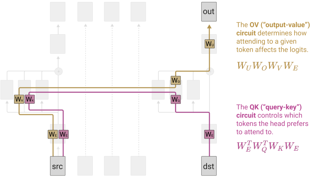
The functional form of an entire attention head is:
where $W_V$ has shape [d_model, d_head], and $W_O$ has shape [d_head, d_model].
Here, we can clearly see that the QK circuit and OV circuit are doing conceptually different things, and should be thought of as two distinct parts of the attention head.
Again, don't worry if you don't follow all of this right now - we'll go into much more detail on all of this in subsequent exercises. The purpose of the discussion here is just to give you a flavour of what's to come!
First, it's useful to visualize and play around with attention patterns - what exactly are we looking at here? (Click on a head to lock onto just showing that head's pattern, it'll make it easier to interpret)
import circuitsvis as cv
from IPython.display import display

display(
    cv.attention.attention_patterns(
        tokens=reference_gpt2.to_str_tokens(reference_text), attention=cache["pattern", 0][0]
    )
)
You can also use the attention_heads function, which presents the data in a different way (the syntax is exactly the same as attention_patterns). Note, if you display this in VSCode then it may exhibit a bug where the main plot continually shrinks in size - if this happens, you should instead save the HTML (i.e. with html = cv.attention.attention_heads(...); with open("attn_heads.html", "w") as f: f.write(str(html))) and open the plot in your browser.
display(
    cv.attention.attention_heads(
        tokens=reference_gpt2.to_str_tokens(reference_text), attention=cache["pattern", 0][0]
    )
)
You should fill in the forward method for Attention below. You should also copy your code for apply_causal_mask to this new implementation of Attention (you can delete the rest of the old implementation code).
Note, this implementation will probably be the most challenging exercise on this page, so don't worry if it takes you some time! You should look at parts of the solution if you're stuck. A few tips:
- Don't forget the attention score scaling (this should come before the masking).
- Try not to combine a large number of operations into a single line of code.
- Try to make your variable names descriptive (i.e. it's not just
x = some_fn_of(x), x = some_other_fn_of(x), ...).
class Attention(nn.Module):
    IGNORE: Float[Tensor, ""]

    def __init__(self, cfg: Config):
        super().__init__()
        self.cfg = cfg
        self.W_Q = nn.Parameter(t.empty((cfg.n_heads, cfg.d_model, cfg.d_head)))
        self.W_K = nn.Parameter(t.empty((cfg.n_heads, cfg.d_model, cfg.d_head)))
        self.W_V = nn.Parameter(t.empty((cfg.n_heads, cfg.d_model, cfg.d_head)))
        self.W_O = nn.Parameter(t.empty((cfg.n_heads, cfg.d_head, cfg.d_model)))
        self.b_Q = nn.Parameter(t.zeros((cfg.n_heads, cfg.d_head)))
        self.b_K = nn.Parameter(t.zeros((cfg.n_heads, cfg.d_head)))
        self.b_V = nn.Parameter(t.zeros((cfg.n_heads, cfg.d_head)))
        self.b_O = nn.Parameter(t.zeros((cfg.d_model)))
        nn.init.normal_(self.W_Q, std=self.cfg.init_range)
        nn.init.normal_(self.W_K, std=self.cfg.init_range)
        nn.init.normal_(self.W_V, std=self.cfg.init_range)
        nn.init.normal_(self.W_O, std=self.cfg.init_range)
        self.register_buffer("IGNORE", t.tensor(float("-inf"), dtype=t.float32, device=device))

    def forward(
        self, normalized_resid_pre: Float[Tensor, "batch posn d_model"]
    ) -> Float[Tensor, "batch posn d_model"]:
        raise NotImplementedError()

    def apply_causal_mask(
        self, attn_scores: Float[Tensor, "batch n_heads query_pos key_pos"]
    ) -> Float[Tensor, "batch n_heads query_pos key_pos"]:
        """
        Applies a causal mask to attention scores, and returns masked scores.
        """
        # You should copy your solution from earlier
        raise NotImplementedError()


tests.test_causal_mask(Attention.apply_causal_mask)
rand_float_test(Attention, [2, 4, 768])
load_gpt2_test(Attention, reference_gpt2.blocks[0].attn, cache["normalized", 0, "ln1"])
Hint (pseudocode for the forward method)
def forward(
    self, normalized_resid_pre: Float[Tensor, "batch posn d_model"]
) -> Float[Tensor, "batch posn d_model"]:
# Calculate query, key and value vectors
    q, k, v = ...
# Calculate attention scores, then scale and mask, and apply softmax to get probabilities
    attn_scores = ...
    attn_scores_masked = ...
    attn_pattern = ...
# Take weighted sum of value vectors, according to attention probabilities
    z = ...
# Calculate output (by applying matrix W_O and summing over heads, then adding bias b_O)
    attn_out = ...
    return attn_out
Solution
class Attention(nn.Module):
    IGNORE: Float[Tensor, ""]
def __init__(self, cfg: Config):
        super().__init__()
        self.cfg = cfg
        self.W_Q = nn.Parameter(t.empty((cfg.n_heads, cfg.d_model, cfg.d_head)))
        self.W_K = nn.Parameter(t.empty((cfg.n_heads, cfg.d_model, cfg.d_head)))
        self.W_V = nn.Parameter(t.empty((cfg.n_heads, cfg.d_model, cfg.d_head)))
        self.W_O = nn.Parameter(t.empty((cfg.n_heads, cfg.d_head, cfg.d_model)))
        self.b_Q = nn.Parameter(t.zeros((cfg.n_heads, cfg.d_head)))
        self.b_K = nn.Parameter(t.zeros((cfg.n_heads, cfg.d_head)))
        self.b_V = nn.Parameter(t.zeros((cfg.n_heads, cfg.d_head)))
        self.b_O = nn.Parameter(t.zeros((cfg.d_model)))
        nn.init.normal_(self.W_Q, std=self.cfg.init_range)
        nn.init.normal_(self.W_K, std=self.cfg.init_range)
        nn.init.normal_(self.W_V, std=self.cfg.init_range)
        nn.init.normal_(self.W_O, std=self.cfg.init_range)
        self.register_buffer("IGNORE", t.tensor(float("-inf"), dtype=t.float32, device=device))
def forward(
        self, normalized_resid_pre: Float[Tensor, "batch posn d_model"]
    ) -> Float[Tensor, "batch posn d_model"]:
        # Calculate query, key and value vectors
        q = (
            einops.einsum(
                normalized_resid_pre,
                self.W_Q,
                "batch posn d_model, nheads d_model d_head -> batch posn nheads d_head",
            )
            + self.b_Q
        )
        k = (
            einops.einsum(
                normalized_resid_pre,
                self.W_K,
                "batch posn d_model, nheads d_model d_head -> batch posn nheads d_head",
            )
            + self.b_K
        )
        v = (
            einops.einsum(
                normalized_resid_pre,
                self.W_V,
                "batch posn d_model, nheads d_model d_head -> batch posn nheads d_head",
            )
            + self.b_V
        )
# Calculate attention scores, then scale and mask, and apply softmax to get probabilities
        attn_scores = einops.einsum(
            q,
            k,
            "batch posn_Q nheads d_head, batch posn_K nheads d_head -> batch nheads posn_Q posn_K",
        )
        attn_scores_masked = self.apply_causal_mask(attn_scores / self.cfg.d_head**0.5)
        attn_pattern = attn_scores_masked.softmax(-1)
# Take weighted sum of value vectors, according to attention probabilities
        z = einops.einsum(
            v,
            attn_pattern,
            "batch posn_K nheads d_head, batch nheads posn_Q posn_K -> batch posn_Q nheads d_head",
        )
# Calculate output (by applying matrix W_O and summing over heads, then adding bias b_O)
        attn_out = (
            einops.einsum(
                z,
                self.W_O,
                "batch posn_Q nheads d_head, nheads d_head d_model -> batch posn_Q d_model",
            )
            + self.b_O
        )
return attn_out
def apply_causal_mask(
        self, attn_scores: Float[Tensor, "batch n_heads query_pos key_pos"]
    ) -> Float[Tensor, "batch n_heads query_pos key_pos"]:
        """
        Applies a causal mask to attention scores, and returns masked scores.
        """
        # Define a mask that is True for all positions we want to set probabilities to zero for
        all_ones = t.ones(attn_scores.size(-2), attn_scores.size(-1), device=attn_scores.device)
        mask = t.triu(all_ones, diagonal=1).bool()
        # Apply the mask to attention scores, then return the masked scores
        attn_scores.masked_fill_(mask, self.IGNORE)
        return attn_scores
Exercise - implement MLP
Next, you should implement the MLP layer, which consists of:
- A linear layer, with weight
W_in, biasb_in - A nonlinear function (we usually use GELU; the function
gelu_newhas been imported for this purpose) - A linear layer, with weight
W_out, biasb_out
class MLP(nn.Module):
    def __init__(self, cfg: Config):
        super().__init__()
        self.cfg = cfg
        self.W_in = nn.Parameter(t.empty((cfg.d_model, cfg.d_mlp)))
        self.W_out = nn.Parameter(t.empty((cfg.d_mlp, cfg.d_model)))
        self.b_in = nn.Parameter(t.zeros((cfg.d_mlp)))
        self.b_out = nn.Parameter(t.zeros((cfg.d_model)))
        nn.init.normal_(self.W_in, std=self.cfg.init_range)
        nn.init.normal_(self.W_out, std=self.cfg.init_range)

    def forward(
        self, normalized_resid_mid: Float[Tensor, "batch posn d_model"]
    ) -> Float[Tensor, "batch posn d_model"]:
        raise NotImplementedError()


rand_float_test(MLP, [2, 4, 768])
load_gpt2_test(MLP, reference_gpt2.blocks[0].mlp, cache["normalized", 0, "ln2"])
Solution
class MLP(nn.Module):
    def __init__(self, cfg: Config):
        super().__init__()
        self.cfg = cfg
        self.W_in = nn.Parameter(t.empty((cfg.d_model, cfg.d_mlp)))
        self.W_out = nn.Parameter(t.empty((cfg.d_mlp, cfg.d_model)))
        self.b_in = nn.Parameter(t.zeros((cfg.d_mlp)))
        self.b_out = nn.Parameter(t.zeros((cfg.d_model)))
        nn.init.normal_(self.W_in, std=self.cfg.init_range)
        nn.init.normal_(self.W_out, std=self.cfg.init_range)
def forward(
        self, normalized_resid_mid: Float[Tensor, "batch posn d_model"]
    ) -> Float[Tensor, "batch posn d_model"]:
        pre = (
            einops.einsum(
                normalized_resid_mid,
                self.W_in,
                "batch position d_model, d_model d_mlp -> batch position d_mlp",
            )
            + self.b_in
        )
        post = gelu_new(pre)
        mlp_out = (
            einops.einsum(
                post, self.W_out, "batch position d_mlp, d_mlp d_model -> batch position d_model"
            )
            + self.b_out
        )
        return mlp_out
Exercise - implement TransformerBlock
Now, we can put together the attention, MLP and layernorms into a single transformer block. Remember to implement the residual connections correctly!
class TransformerBlock(nn.Module):
    def __init__(self, cfg: Config):
        super().__init__()
        self.cfg = cfg
        self.ln1 = LayerNorm(cfg)
        self.attn = Attention(cfg)
        self.ln2 = LayerNorm(cfg)
        self.mlp = MLP(cfg)

    def forward(
        self, resid_pre: Float[Tensor, "batch position d_model"]
    ) -> Float[Tensor, "batch position d_model"]:
        raise NotImplementedError()


rand_float_test(TransformerBlock, [2, 4, 768])
load_gpt2_test(TransformerBlock, reference_gpt2.blocks[0], cache["resid_pre", 0])
Help - I'm getting 100% accuracy on all modules before this point, but only about 90% accuracy on this one.
This might be because your layernorm implementation divides by std + eps rather than (var + eps).sqrt(). The latter matches the implementation used by GPT-2 (and this error only shows up in these tests).
Solution
class TransformerBlock(nn.Module):
    def __init__(self, cfg: Config):
        super().__init__()
        self.cfg = cfg
        self.ln1 = LayerNorm(cfg)
        self.attn = Attention(cfg)
        self.ln2 = LayerNorm(cfg)
        self.mlp = MLP(cfg)
def forward(
        self, resid_pre: Float[Tensor, "batch position d_model"]
    ) -> Float[Tensor, "batch position d_model"]:
        resid_mid = self.attn(self.ln1(resid_pre)) + resid_pre
        resid_post = self.mlp(self.ln2(resid_mid)) + resid_mid
        return resid_post
Exercise - implement Unembed
The unembedding is just a linear layer (with weight W_U and bias b_U).
class Unembed(nn.Module):
    def __init__(self, cfg):
        super().__init__()
        self.cfg = cfg
        self.W_U = nn.Parameter(t.empty((cfg.d_model, cfg.d_vocab)))
        nn.init.normal_(self.W_U, std=self.cfg.init_range)
        self.b_U = nn.Parameter(t.zeros((cfg.d_vocab), requires_grad=False))

    def forward(
        self, normalized_resid_final: Float[Tensor, "batch position d_model"]
    ) -> Float[Tensor, "batch position d_vocab"]:
        raise NotImplementedError()


rand_float_test(Unembed, [2, 4, 768])
load_gpt2_test(Unembed, reference_gpt2.unembed, cache["ln_final.hook_normalized"])
Solution
class Unembed(nn.Module):
    def __init__(self, cfg):
        super().__init__()
        self.cfg = cfg
        self.W_U = nn.Parameter(t.empty((cfg.d_model, cfg.d_vocab)))
        nn.init.normal_(self.W_U, std=self.cfg.init_range)
        self.b_U = nn.Parameter(t.zeros((cfg.d_vocab), requires_grad=False))
def forward(
        self, normalized_resid_final: Float[Tensor, "batch position d_model"]
    ) -> Float[Tensor, "batch position d_vocab"]:
        return (
            einops.einsum(
                normalized_resid_final,
                self.W_U,
                "batch posn d_model, d_model d_vocab -> batch posn d_vocab",
            )
            + self.b_U
        )
Exercise - implement DemoTransformer
class DemoTransformer(nn.Module):
    def __init__(self, cfg: Config):
        super().__init__()
        self.cfg = cfg
        self.embed = Embed(cfg)
        self.pos_embed = PosEmbed(cfg)
        self.blocks = nn.ModuleList([TransformerBlock(cfg) for _ in range(cfg.n_layers)])
        self.ln_final = LayerNorm(cfg)
        self.unembed = Unembed(cfg)

    def forward(
        self, tokens: Int[Tensor, "batch position"]
    ) -> Float[Tensor, "batch position d_vocab"]:
        raise NotImplementedError()


rand_int_test(DemoTransformer, [2, 4])
load_gpt2_test(DemoTransformer, reference_gpt2, tokens)
Solution
class DemoTransformer(nn.Module):
    def __init__(self, cfg: Config):
        super().__init__()
        self.cfg = cfg
        self.embed = Embed(cfg)
        self.pos_embed = PosEmbed(cfg)
        self.blocks = nn.ModuleList([TransformerBlock(cfg) for _ in range(cfg.n_layers)])
        self.ln_final = LayerNorm(cfg)
        self.unembed = Unembed(cfg)
def forward(
        self, tokens: Int[Tensor, "batch position"]
    ) -> Float[Tensor, "batch position d_vocab"]:
        residual = self.embed(tokens) + self.pos_embed(tokens)
        for block in self.blocks:
            residual = block(residual)
        logits = self.unembed(self.ln_final(residual))
        return logits
Try it out!
demo_gpt2 = DemoTransformer(Config(debug=False)).to(device)
demo_gpt2.load_state_dict(reference_gpt2.state_dict(), strict=False)

demo_logits = demo_gpt2(tokens)
Let's take a test string, and calculate the loss!
We're using the formula for cross-entropy loss. The cross entropy loss between a modelled distribution $Q$ and target distribution $P$ is:
In the case where $P$ is just the empirical distribution from target classes (i.e. $P(x^*) = 1$ for the correct class $x^*$) then this becomes:
in other words, the negative log prob of the true classification.
def get_log_probs(
    logits: Float[Tensor, "batch posn d_vocab"], tokens: Int[Tensor, "batch posn"]
) -> Float[Tensor, "batch posn-1"]:
    log_probs = logits.log_softmax(dim=-1)
    # Get logprobs the first seq_len-1 predictions (so we can compare them with the actual next tokens)
    log_probs_for_tokens = (
        log_probs[:, :-1].gather(dim=-1, index=tokens[:, 1:].unsqueeze(-1)).squeeze(-1)
    )

    return log_probs_for_tokens


pred_log_probs = get_log_probs(demo_logits, tokens)
print(f"Avg cross entropy loss: {-pred_log_probs.mean():.4f}")
print(f"Avg cross entropy loss for uniform distribution: {math.log(demo_gpt2.cfg.d_vocab):4f}")
print(f"Avg probability assigned to correct token: {pred_log_probs.exp().mean():4f}")
Avg cross entropy loss: 4.0441
Avg cross entropy loss for uniform distribution: 10.824905
Avg probability assigned to correct token: 0.098628
We can also greedily generate text, by taking the most likely next token and continually appending it to our prompt before feeding it back into the model:
test_string = """Mitigating the risk of extinction from AI should be a global priority alongside other societal-scale risks such as"""
for i in tqdm(range(100)):
    test_tokens = reference_gpt2.to_tokens(test_string).to(device)
    demo_logits = demo_gpt2(test_tokens)
    test_string += reference_gpt2.tokenizer.decode(demo_logits[-1, -1].argmax())

print(test_string)
Mitigating the risk of extinction from AI should be a global priority alongside other societal-scale risks such as climate change, the spread of infectious diseases and the spread of infectious diseases.

The research is published in the journal Nature Communications.

The research team is led by Dr. Michael J. H. Haldane, a professor of biology at the University of California, Berkeley, and co-author of the paper.

"We are very excited to see that the AI community is starting to take notice of the potential for AI to be a major threat to the human race,"
In section 4️⃣ we'll learn to generate text in slightly more interesting ways than just argmaxing the output (which can lead to unnatural patterns like repetition, or text which is just less natural-sounding).