1️⃣ Autoencoders & VAEs
Learning Objectives
- Learn about the transposed convolution operation
- Understand the basic architecture of autoencoders and VAEs
- Learn about the reparameterization trick for VAEs
- Implement your own autoencoder
- Implement your own VAE, and use it to generate realistic MNIST images
- (optional) Dive deeper into the mathematical underpinnings of VAEs, and learn about the ELBO loss function
Reading
Note - before you start the reading, you might want to run the first block of code in the "Loading data" section, because it can take a few minutes to run.
- Understanding VAEs (Medium)
- A clear and accessible explanation of autoencoders and VAEs.
- You can stop at "Mathematical details of VAEs"; we'll (optionally) cover this in more detail later.
- Six (and a half) intuitions for KL divergence
- Optional reading.
- KL divergence is an important concept in VAEs (and will continue to be a useful concept for the rest of this course).
- From Autoencoder to Beta-VAE
- Optional reading.
- This is a more in-depth look at VAEs, the maths behind them, and different architecture variants.
- Transposed Convolutions explained with… MS Excel! (optional)
- Optional reading.
- The first part (up to the highlighted comment) is most valuable, since understanding transposed convolutions at a high level is more important than understanding the exact low-level operations that go into them (that's what the bonus is for!).
- These visualisations may also help.
Loading data
In these exercises, we'll be using either the Celeb-A dataset or the MNIST dataset. For convenience, we'll include a few functions here to load that data in.
You should already be familiar with MNIST. You can read about the Celeb-A dataset here - essentially it's a large-scale face attributes dataset with more than 200k celebrity images, but we'll only be taking the images from this dataset rather the classifications. Run the code below to download the data from HuggingFace, and save it in your filesystem as images.
The code should take 4-15 minutes to run in total, but feel free to move on if it's taking longer (you'll mostly be using MNIST in this section, and only using Celeb-A when you move on to GANs).
celeb_data_dir = section_dir / "data/celeba"
celeb_image_dir = celeb_data_dir / "img_align_celeba"

os.makedirs(celeb_image_dir, exist_ok=True)

if len(list(celeb_image_dir.glob("*.jpg"))) > 0:
    print("Dataset already loaded.")
else:
    dataset = load_dataset("nielsr/CelebA-faces")
    print("Dataset loaded.")

    for idx, item in tqdm(
        enumerate(dataset["train"]), total=len(dataset["train"]), desc="Saving imgs...", ascii=True
    ):
        # The image is already a JpegImageFile, so we can directly save it
        item["image"].save(celeb_image_dir / f"{idx:06}.jpg")

    print("All images have been saved.")
Note on why we double-nest our saving paths, i.e. celeba/img_align_celeba
In the code above, each image is saved in the format 'data/celeba/img_align_celeba/000001.jpg', etc. The reason for this double nesting (rather than e.g. data/celeba/000001.jpg) is that the child folders represent the image classes. If we were training a classifier, we'd have multiple folders within data/celeba, with each one being a different class. In this dataset, we only have one class (real celeb images), so we only need one child folder.
Now, here's some code to load in either the Celeb-A or MNIST data. It also applies transformations to the data, to get it into the right input format for us.
The function below allows you to load in either the Celeb-A or MNIST data.
def get_dataset(dataset: Literal["MNIST", "CELEB"], train: bool = True) -> Dataset:
    assert dataset in ["MNIST", "CELEB"]

    if dataset == "CELEB":
        image_size = 64
        assert train, "CelebA dataset only has a training set"
        transform = transforms.Compose(
            [
                transforms.Resize(image_size),
                transforms.CenterCrop(image_size),
                transforms.ToTensor(),
                transforms.Normalize((0.5, 0.5, 0.5), (0.5, 0.5, 0.5)),
            ]
        )
        trainset = datasets.ImageFolder(
            root=exercises_dir / "part5_vaes_and_gans/data/celeba", transform=transform
        )

    elif dataset == "MNIST":
        img_size = 28
        transform = transforms.Compose(
            [
                transforms.Resize(img_size),
                transforms.ToTensor(),
                transforms.Normalize((0.1307,), (0.3081,)),
            ]
        )
        trainset = datasets.MNIST(
            root=exercises_dir / "part5_vaes_and_gans/data",
            transform=transform,
            download=True,
            train=train,
        )

    return trainset
We've also given you some code for visualising your data. You should run this code to make sure your data is correctly loaded in.
def display_data(x: Tensor, nrows: int, title: str):
    """Displays a batch of data, using plotly."""
    ncols = x.shape[0] // nrows
    # Reshape into the right shape for plotting (make it 2D if image is monochrome)
    y = einops.rearrange(x, "(b1 b2) c h w -> (b1 h) (b2 w) c", b1=nrows).squeeze()
    # Normalize in the 0-1 range, then map to integer type
    y = (y - y.min()) / (y.max() - y.min())
    y = (y * 255).to(dtype=t.uint8)
    # Display data
    imshow(
        y,
        binary_string=(y.ndim == 2),
        height=50 * (nrows + 4),
        width=50 * (ncols + 5),
        title=f"{title}<br>single input shape = {x[0].shape}",
    )


trainset_mnist = get_dataset("MNIST")
trainset_celeb = get_dataset("CELEB")

# Display MNIST
x = next(iter(DataLoader(trainset_mnist, batch_size=25)))[0]
display_data(x, nrows=5, title="MNIST data")

# Display CelebA
x = next(iter(DataLoader(trainset_celeb, batch_size=25)))[0]
display_data(x, nrows=5, title="CelebA data")
Holdout data
Lastly, we'll also get some holdout data that we can use during training. The tensor below has shape (10, 1, 28, 28), and contains a single image from each of the 10 MNIST classes. We do this because we want to monitor our autoencoder's reconstructions for each different image type while it trains. We might find that some images are reconstructed better than others!
testset = get_dataset("MNIST", train=False)
HOLDOUT_DATA = dict()
for data, target in DataLoader(testset, batch_size=1):
    if target.item() not in HOLDOUT_DATA:
        HOLDOUT_DATA[target.item()] = data.squeeze()
        if len(HOLDOUT_DATA) == 10:
            break
HOLDOUT_DATA = (
    t.stack([HOLDOUT_DATA[i] for i in range(10)]).to(dtype=t.float, device=device).unsqueeze(1)
)

display_data(HOLDOUT_DATA, nrows=1, title="MNIST holdout data")
You might be wondering why we do this, rather than just e.g. generating some random noise and seeing what the decoder's reconstruction is. The answer is that our autoencoder's latent space might not be meaningful. In other words, it's unclear exactly how to sample from it to get output which will look like an MNIST image. We'll return to this idea when we study VAEs later in these exercises.
For the rest of this section (not including the bonus), we'll assume we're working with the MNIST dataset rather than Celeb-A.
Transposed Convolutions
What are transposed convolutions, and why should we care about them? One high-level intuition goes something like this: most of the generator's architecture is basically the discriminator architecture in reverse. We need something that performs the reverse of a convolution - not literally the inverse operation, but something reverse in spirit, which uses a kernel of weights to project up to some array of larger size.
Importantly, a transposed convolution isn't literally the inverse of a convolution. A lot of confusion can come from misunderstanding this!
You can describe the difference between convolutions and transposed convolutions as follows:
- In convolutions, you slide the kernel around inside the input. At each position of the kernel, you take a sumproduct between the kernel and that section of the input to calculate a single element in the output.
- In transposed convolutions, you slide the kernel around what will eventually be your output, and at each position you add some multiple of the kernel to your output.
Below is an illustration of both for comparison, in the 1D case (where $*$ stands for the 1D convolution operator, and $*^T$ stands for the transposed convolution operator). Note the difference in size between the output in both cases. With standard convolutions, our output is smaller than our input, because we're having to fit the kernel inside the input in order to produce the output. But in our transposed convolutions, the output is actually larger than the input, because we're fitting the kernel inside the output.
![]()
We won't actually have you implement the transposed convolution operation in these exercises; instead we've pushed it to the bonus section. For now, you can just use the ConvTranspose2d module which has already been imported for you from today's solutions file, in place of your own implementation. You can use it exactly the same way you use normal convolutional layers: for instance ConvTranspose2d(32, 16, 4, stride=2, padding=1) will define a convolution layer that maps a tensor from (batch_size, in_channels=32, height, width) up to shape (batch_size, out_channels=16, height * 2, width * 2).
These visualisations (linked in the reading material) may also help build intuition for the transposed convolution module.
Autoencoders
We'll start by looking at Autoencoders, which are much conceptually simpler than VAEs. These are simply systems which learn a compressed representation of the input, and then reconstruct it. There are two parts to this:
- The encoder learns to compress the output into a latent space which is lower-dimensional than the original image.
- The decoder learns to uncompress the encoder's output back into a faithful representation of the original image.
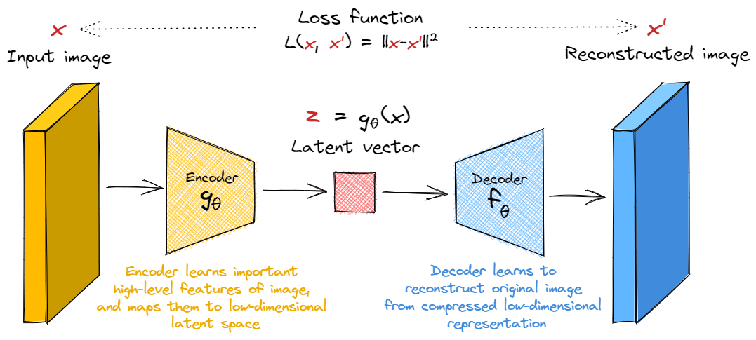
Our loss function is simply some metric of the distance between the input and the reconstructed input, e.g. the $l_2$ loss.
You'll start by writing your own autoencoder. We've given some guidance on architecture below, although in general because we're working with a fairly simple dataset (MNIST) and a fairly robust architecture (at least compared to GANs in the next section!), you model is still likely to work well even if it deviates slightly from the specification we'll give below.
Exercise - implement autoencoder
```yaml Difficulty: 🔴🔴🔴⚪⚪ Importance: 🔵🔵🔵🔵⚪
You should spend up to 15-30 minutes on this exercise. ```
Note - for the rest of this section (not including the bonus), we'll assume we're working with the MNIST dataset rather than Celeb-A.
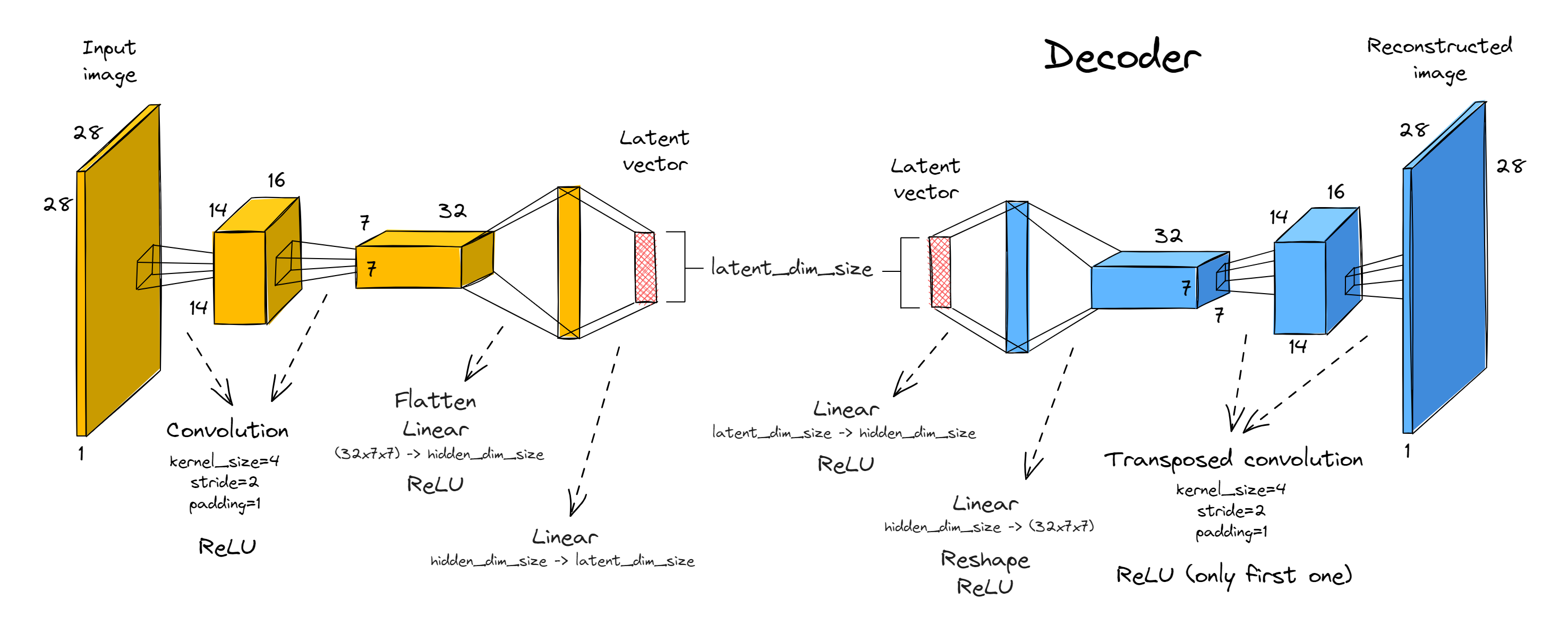
Your encoder should consist of two convolutional blocks (i.e. convolution plus ReLU), followed by two fully connected linear layers with a ReLU in between them. Both convolutions will have kernel size 4, stride 2, padding 1 (recall this halves the size of the image). We'll have 16 and 32 output channels respectively.
The decoder will be the exact mirror image of the encoder (with convolutions replaced by transposed convolutions).
The only free parameters in your implementation will be latent_dim_size and hidden_dim_size. The former determines the size of the latent space (otherwise called the bottleneck dimension) between the encoder and decoder, and the latter determines the size of the final linear layer we insert just before the end / just after the start of the encoder / decoder's architecture respectively.
A few extra notes:
- You'll need to reshape between the convolutional blocks and linear layers. For this, you might find the
einopslibrary helpful - they have a functioneinops.layers.torch.Rearrange(imported for you asRearrange) which works like the standard einops function, except that it takes a string and returns a module which performs the corresponding rearrangement. Just like any other module, it can be used inside things likeSequential(this way, the logic inside theforwardmethod can be very simple!).
>>> x = t.randn(100, 3, 4, 5)
>>> x.shape
torch.Size([100, 3, 4, 5])

>>> module = Rearrange("b c h w -> b (c h w)")
>>> module(x).shape
torch.Size([100, 60])
- Note that we don't include a ReLU in the very last layer of the decoder or generator, we only include them between successive convolutions or linear layers - can you see why it wouldn't make sense to put ReLUs at the end?
- The convolutions don't have biases, although we have included biases in the linear layers (this will be important if you want your parameter count to match the solution, but not really that important for good performance).
Now, implement your autoencoder below. We recommend you define encoder and decoder to help make your code run with the functions we've written for you later.
# Importing all modules you'll need, from previous solutions (you're encouraged to substitute your
# own implementations instead, if you want to!)
from part2_cnns.solutions import BatchNorm2d, Conv2d, Linear, ReLU, Sequential

from part5_vaes_and_gans.solutions import ConvTranspose2d


class Autoencoder(nn.Module):
    def __init__(self, latent_dim_size: int, hidden_dim_size: int):
        """Creates the encoder & decoder modules."""
        super().__init__()
        self.encoder = ...
        self.decoder = ...

    def forward(self, x: Tensor) -> Tensor:
        """Returns the reconstruction of the input, after mapping through encoder & decoder."""
        raise NotImplementedError()


tests.test_autoencoder(Autoencoder)
Solution
class Autoencoder(nn.Module):
    def __init__(self, latent_dim_size: int, hidden_dim_size: int):
        """Creates the encoder & decoder modules."""
        super().__init__()
        self.latent_dim_size = latent_dim_size
        self.hidden_dim_size = hidden_dim_size
        self.encoder = Sequential(
            Conv2d(1, 16, 4, stride=2, padding=1),
            ReLU(),
            Conv2d(16, 32, 4, stride=2, padding=1),
            ReLU(),
            Rearrange("b c h w -> b (c h w)"),
            Linear(7  7  32, hidden_dim_size),
            ReLU(),
            Linear(hidden_dim_size, latent_dim_size),
        )
        self.decoder = nn.Sequential(
            Linear(latent_dim_size, hidden_dim_size),
            ReLU(),
            Linear(hidden_dim_size, 7  7  32),
            ReLU(),
            Rearrange("b (c h w) -> b c h w", c=32, h=7, w=7),
            ConvTranspose2d(32, 16, 4, stride=2, padding=1),
            ReLU(),
            ConvTranspose2d(16, 1, 4, stride=2, padding=1),
        )
def forward(self, x: Tensor) -> Tensor:
        """Returns the reconstruction of the input, after mapping through encoder & decoder."""
        z = self.encoder(x)
        x_prime = self.decoder(z)
        return x_prime
Training your Autoencoder
Once you've got the architecture right, you should write a training loop which works with MSE loss between the original and reconstructed data. The standard Adam optimiser with default parameters should suffice.
Logging images to wandb
Weights and biases provides a nice feature allowing you to log images! This requires you to use the function wandb.Image. The first argument is data_or_path, which can be any of the following:
- A numpy array in shape
(height, width)or(height, width, 1)-> interpreted as monochrome image - A numpy array in shape
(height, width, 3)-> interpreted as RGB image - A PIL image (can be RGB or monochrome)
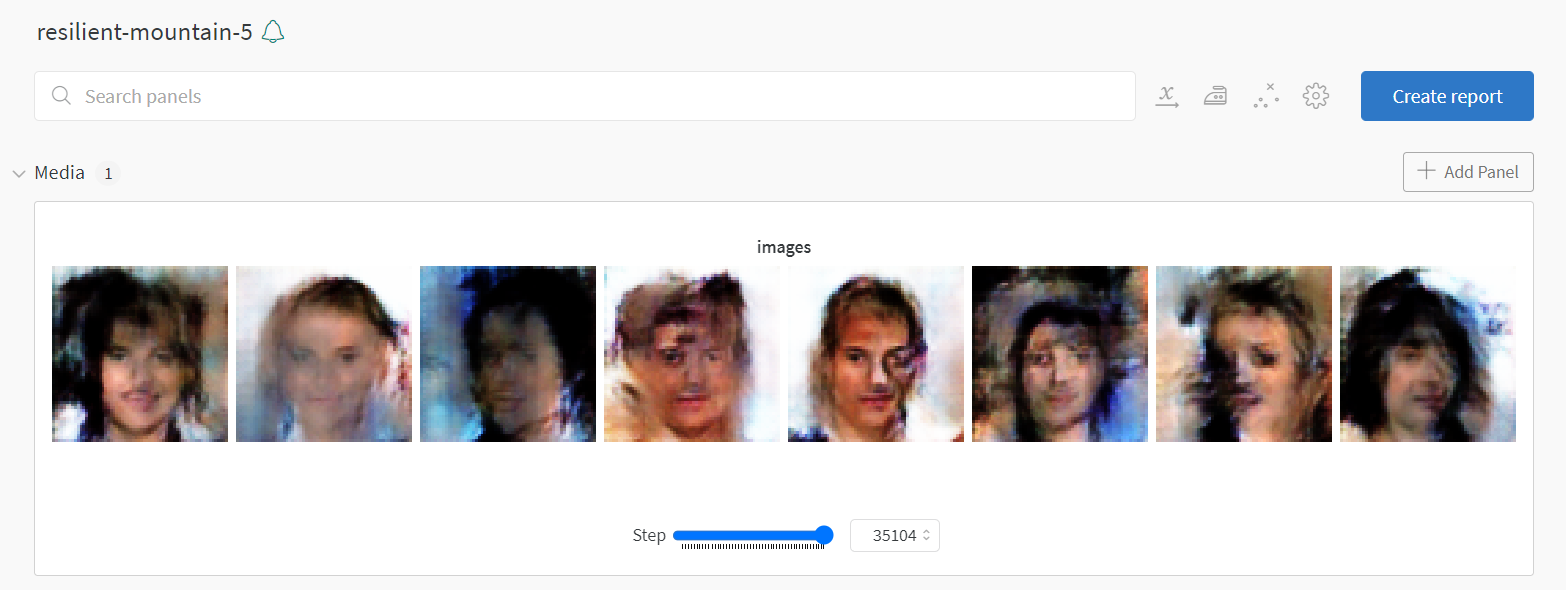
When it comes to logging, you can log a list of images rather than a single image. Example code, and the output it produces from my GAN (you'll create output like this in the next section!):
# arr is a numpy array of shape (8, 28, 28, 3), i.e. it's an array of 8 RGB images
images = [wandb.Image(a) for a in arr]
wandb.log({"images": images}, step=self.step)
Exercise - write autoencoder training loop
```yaml Difficulty: 🔴🔴🔴🔴⚪ Importance: 🔵🔵🔵🔵⚪
You should spend up to 20-35 minutes on this exercise. ```
You should now implement your training loop below. We've filled in some methods for you (and have given you a dataclass to hold arguments), your job is to complete training_step and train. The former should perform a single training step by optimizing against the reconstruction loss between the image and target (you might find nn.MSELoss suitable for this). The latter should be structured like training code you might have seen before, in other words:
- Iterate over
self.args.epochsepochs - For each epoch, you should:
- Iterate over the training data and perform a training step for each batch. We also recommend using & updating a progress bar, and logging to wandb if this is enabled in your training arguments.
- Evaluate the model on the holdout data via
self.log_samples(), everyargs.log_every_n_stepstotal steps.
Some last tips before we get started:
- Don't use wandb until you've ironed out the bugs in your code, and loss seems to be going down based on the in-notebook logging. This is why we've given you the
use_wandbargument in your dataclass. - Remember to increment
self.stepas you train (this is necessary if you're passing this argument towandb.log). Note we're usingstephere rather thanexamples_seenlike in earlier exercises, because it'll prove more useful for our purposes. - Your wandb logging should take place in
training_stepnottrain(this is better practice in general because often there will be variables only defined in the scope oftraining_stepthat you might want to log - even though that's not the case here, it will be later). - Iterating through
self.trainloaderwill give you tuples of(img, label), but you don't need to use the labels - all you need is the image.
@dataclass
class AutoencoderArgs:
    # architecture
    latent_dim_size: int = 5
    hidden_dim_size: int = 128

    # data / training
    dataset: Literal["MNIST", "CELEB"] = "MNIST"
    batch_size: int = 512
    epochs: int = 10
    lr: float = 1e-3
    betas: tuple[float, float] = (0.5, 0.999)

    # logging
    use_wandb: bool = True
    wandb_project: str | None = "day5-autoencoder"
    wandb_name: str | None = None
    log_every_n_steps: int = 250


class AutoencoderTrainer:
    def __init__(self, args: AutoencoderArgs):
        self.args = args
        self.trainset = get_dataset(args.dataset)
        self.trainloader = DataLoader(self.trainset, batch_size=args.batch_size, shuffle=True)
        self.model = Autoencoder(
            latent_dim_size=args.latent_dim_size,
            hidden_dim_size=args.hidden_dim_size,
        ).to(device)
        self.optimizer = t.optim.Adam(self.model.parameters(), lr=args.lr, betas=args.betas)

    def training_step(self, img: Tensor) -> Tensor:
        """
        Performs a training step on the batch of images in `img`. Returns the loss. Logs to wandb
        if enabled.
        """
        raise NotImplementedError()

    @t.inference_mode()
    def log_samples(self) -> None:
        """
        Evaluates model on holdout data, either logging to weights & biases or displaying output.
        """
        assert self.step > 0, (
            "First call should come after a training step. Remember to increment `self.step`."
        )
        output = self.model(HOLDOUT_DATA)
        if self.args.use_wandb:
            output = (output - output.min()) / (output.max() - output.min())  # Normalize to [0, 1]
            output = (output * 255).to(dtype=t.uint8)  # Convert to uint8 for logging
            wandb.log(
                {"images": [wandb.Image(arr) for arr in output.cpu().numpy()]}, step=self.step
            )
        else:
            display_data(t.concat([HOLDOUT_DATA, output]), nrows=2, title="AE reconstructions")

    def train(self) -> Autoencoder:
        """Performs a full training run."""
        self.step = 0
        if self.args.use_wandb:
            wandb.init(project=self.args.wandb_project, name=self.args.wandb_name)
            wandb.watch(self.model)

        # YOUR CODE HERE - iterate over epochs, and train your model

        if self.args.use_wandb:
            wandb.finish()

        return self.model


args = AutoencoderArgs(use_wandb=False)
trainer = AutoencoderTrainer(args)
autoencoder = trainer.train()
Solution
class AutoencoderTrainer:
    def __init__(self, args: AutoencoderArgs):
        self.args = args
        self.trainset = get_dataset(args.dataset)
        self.trainloader = DataLoader(self.trainset, batch_size=args.batch_size, shuffle=True)
        self.model = Autoencoder(
            latent_dim_size=args.latent_dim_size,
            hidden_dim_size=args.hidden_dim_size,
        ).to(device)
        self.optimizer = t.optim.Adam(self.model.parameters(), lr=args.lr, betas=args.betas)
def training_step(self, img: Tensor) -> Tensor:
        """
        Performs a training step on the batch of images in img. Returns the loss. Logs to wandb
        if enabled.
        """
        # Compute loss, backprop on it, and perform an optimizer step
        img_reconstructed = self.model(img)
        loss = nn.MSELoss()(img, img_reconstructed)
        loss.backward()
        self.optimizer.step()
        self.optimizer.zero_grad()
# Increment step counter and log to wandb if enabled
        self.step += img.shape[0]
        if self.args.use_wandb:
            wandb.log(dict(loss=loss), step=self.step)
return loss
@t.inference_mode()
    def log_samples(self) -> None:
        """
        Evaluates model on holdout data, either logging to weights & biases or displaying output.
        """
        assert self.step > 0, (
            "First call should come after a training step. Remember to increment self.step."
        )
        output = self.model(HOLDOUT_DATA)
        if self.args.use_wandb:
            output = (output - output.min()) / (output.max() - output.min())  # Normalize to [0, 1]
            output = (output * 255).to(dtype=t.uint8)  # Convert to uint8 for logging
            wandb.log(
                {"images": [wandb.Image(arr) for arr in output.cpu().numpy()]}, step=self.step
            )
        else:
            display_data(t.concat([HOLDOUT_DATA, output]), nrows=2, title="AE reconstructions")
def train(self) -> Autoencoder:
        """Performs a full training run."""
        self.step = 0
        if self.args.use_wandb:
            wandb.init(project=self.args.wandb_project, name=self.args.wandb_name)
            wandb.watch(self.model)
for epoch in range(self.args.epochs):
            # Iterate over training data, performing a training step for each batch
            progress_bar = tqdm(self.trainloader, total=int(len(self.trainloader)), ascii=True)
            for img, label in progress_bar:  # remember that label is not used
                img = img.to(device)
                loss = self.training_step(img)
                progress_bar.set_description(f"{epoch=:02d}, {loss=:.4f}, step={self.step:05d}")
                if self.step % self.args.log_every_n_steps == 0:
                    self.log_samples()
if self.args.use_wandb:
            wandb.finish()
return self.model
After the first epoch, you should be able to get output of the following quality:
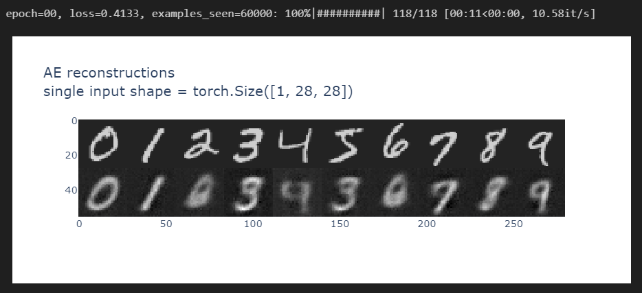
And by the 10th epoch, you should be getting something like this:
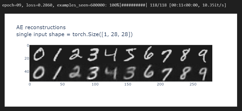
Note how the reconstructions it's mixing up features for some of the numbers - for instance, the 5 seems to have been partly reconstructed as a 3. But overall, it seems pretty accurate!
Latent space of an autoencoder
We'll now return to the issue we mentioned briefly earlier - how to generate output? We might want to generate output by just producing random noise and passing it through our decoder, but this raises a question - how should we interpret the latent space between our encoder and decoder?
We can try and plot the outputs produced by the decoder over a range. The code below does this (you might have to adjust it slightly depending on how you've implemented your autoencoder):
def create_grid_of_latents(
    model, interpolation_range=(-1, 1), n_points=11, dims=(0, 1)
) -> Float[Tensor, "rows_x_cols latent_dims"]:
    """Create a tensor of zeros which varies along the 2 specified dimensions of the latent space."""
    grid_latent = t.zeros(n_points, n_points, model.latent_dim_size, device=device)
    x = t.linspace(*interpolation_range, n_points)
    grid_latent[..., dims[0]] = x.unsqueeze(-1)  # rows vary over dim=0
    grid_latent[..., dims[1]] = x  # cols vary over dim=1
    return grid_latent.flatten(0, 1)  # flatten over (rows, cols) into a single batch dimension


grid_latent = create_grid_of_latents(autoencoder, interpolation_range=(-3, 3))

# Map grid latent through the decoder
output = autoencoder.decoder(grid_latent)

# Visualize the output
utils.visualise_output(output, grid_latent, title="Autoencoder latent space visualization")
Click to see the expected output
This code generates images from a vector in the latent space which is zero in all directions, except for the first two dimensions. (Note, we normalize with (0.3081, 0.1307) in the code above because this is the mean and standard deviation of the MNIST dataset - see discussion here.)
This is ... pretty underwhelming. Some of these shapes seem legible in some regions (e.g. in the demo example on Streamlit we have some patchy but still recognisable 9s, 3s, 0s and 4s in the corners of the latent space), but a lot of the space doesn't look like any recognisable number. For example, much of the middle region is just an unrecognisable blob. Using the default interpolation range of (-1, 1) makes things look even worse. And this is a problem, since our goal is to be able to randomly sample points inside this latent space and use them to generate output which resembles the MNIST dataset - this is our true goal, not accurate reconstruction.
Why does this happen? Well unfortunately, the model has no reason to treat the latent space in any meaningful way. It might be the case that almost all the images are embedded into a particular subspace of the latent space, and so the encoder only gets trained on inputs in this subspace. To further illustrate this, the code below feeds MNIST data into your encoder, and plots the resulting latent vectors (projected along the first two latent dimensions). Note that there are some very high-density spots, and other much lower-density spots. So it stands to reason that we shouldn't expect the decoder to be able to produce good output for all points in the latent space (especially when we're using a 5-dimensional latent space rather than just 2-dimensional as visualised below - we can imagine that 5D latent space would have significantly more "dead space").
To emphasise, we're not looking for a crisp separation of digits here. We're only plotting 2 of 5 dimensions, it would be a coincidence if they were cleanly separated. We're looking for efficient use of the space, because this is likely to lead to an effective generator when taken out of the context of the discriminator. We don't really see that here.
# Get a small dataset with 5000 points
small_dataset = Subset(get_dataset("MNIST"), indices=range(0, 5000))
imgs = t.stack([img for img, label in small_dataset]).to(device)
labels = t.tensor([label for img, label in small_dataset]).to(device).int()

# Get the latent vectors for this data along first 2 dims, plus for the holdout data
latent_vectors = autoencoder.encoder(imgs)[:, :2]
holdout_latent_vectors = autoencoder.encoder(HOLDOUT_DATA)[:, :2]

# Plot the results
utils.visualise_input(latent_vectors, labels, holdout_latent_vectors, HOLDOUT_DATA)
Click to see the expected output
Variational Autoencoders
Variational autoencoders try and solve the problem posed by autoencoders: how to actually make the latent space meaningful, such that you can generate output by feeding a $N(0, 1)$ random vector into your model's decoder?
The key perspective shift is this: rather than mapping the input into a fixed vector, we map it into a distribution. The way we learn a distribution is very similar to the way we learn our fixed inputs for the autoencoder, i.e. we have a bunch of linear or convolutional layers, our input is the original image, and our output is the tuple of parameters $(\mu(\boldsymbol{x}), \Sigma(\boldsymbol{x}))$ (as a trivial example, our VAE learning a distribution $\mu(\boldsymbol{x})=z(\boldsymbol{x})$, $\Sigma(\boldsymbol{x})=0$ is equivalent to our autoencoder learning the function $z(\boldsymbol{x})$ as its encoder).
From this TowardsDataScience article:
Due to overfitting, the latent space of an autoencoder can be extremely irregular (close points in latent space can give very different decoded data, some point of the latent space can give meaningless content once decoded) and, so, we can’t really define a generative process that simply consists to sample a point from the latent space and make it go through the decoder to get new data. Variational autoencoders (VAEs) are autoencoders that tackle the problem of the latent space irregularity by making the encoder return a distribution over the latent space instead of a single point and by adding in the loss function a regularisation term over that returned distribution in order to ensure a better organisation of the latent space.
Or, in fewer words:
A variational autoencoder can be defined as being an autoencoder whose training is regularised to avoid overfitting and ensure that the latent space has good properties that enable generative process.
At first, this idea of mapping to a distribution sounds like a crazy hack - why on earth does it work? This diagram should help convey some of the intuitions:
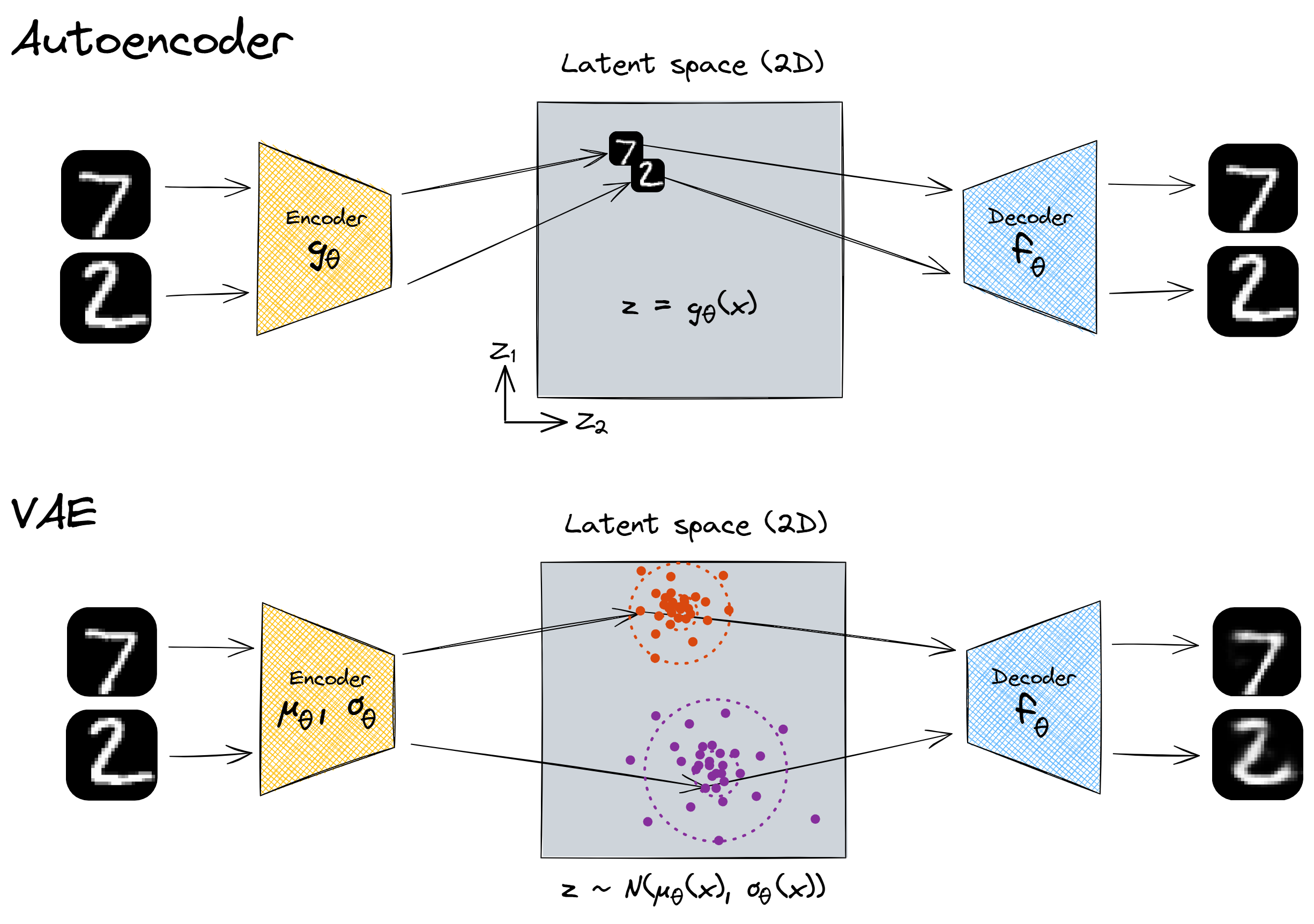
With our encoder, there was nothing incentivising us to make full and meaningful use of the latent space. It's hypothetically possible that our network was mapping all the inputs to some very small subspace and reconstructing them with perfect fidelity. This wouldn't have required numbers with different features to be far apart from each other in the latent space, because even if they are close together no information is lost. See the first image above.
But with our variational autoencoder, each MNIST image produces a sample from the latent space, with a certain mean and variance. This means that, when two numbers look very different, their latent vectors are forced apart - if the means were close together then the decoder wouldn't be able to reconstruct them.
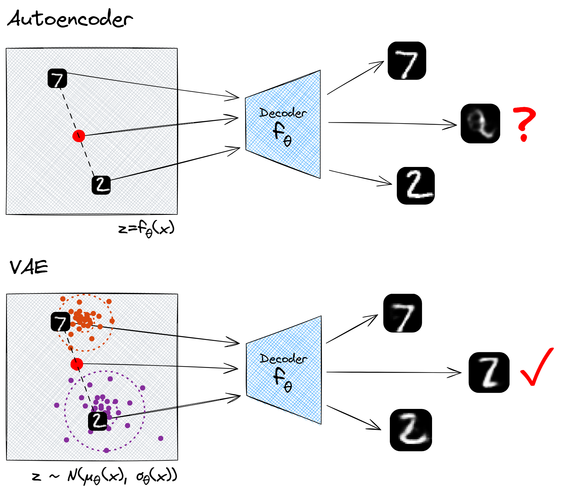
Another nice property of using random latent vectors is that the entire latent space will be meaningful. For instance, with autoencoders there is no reason why we should expect the linear interpolation between two points in the latent space to have meaningful decodings. The decoder output will change continuously as we continuously vary the latent vector, but that's about all we can say about it. However, if we use a variational autoencoder, we don't have this problem. The output of a linear interpolation between the cluster of $2$s and cluster of $7$s will be "a symbol which pattern-matches to the family of MNIST digits, but has equal probability to be interpreted as a $2$ or a $7$", and this is indeed what we find.
Reparameterisation trick
One question that might have occurred to you - how can we perform backward passes through our network? We know how to differentiate with respect to the inputs to a function, but how can we differentiate wrt the parameters of a probability distribution from which we sample our vector? The solution is to convert our random sampling into a function, by introducing an extra parameter $\epsilon$. We sample $\epsilon$ from the standard normal distribution, and then express $\boldsymbol{z}$ as a deterministic function of $\mu$, $\sigma$ and $\epsilon$:
where $\odot$ is a notation meaning pointwise product, i.e. $z_i = \mu_i + \sigma_i \epsilon_i$. Intuitively, we can think of this as follows: when there is randomness in the process that generates the output, there is also randomness in the derivative of the output wrt the input, so we can get a value for the derivative by sampling from this random distribution. If we average over enough samples, this will give us a valid gradient for training.
Note that if we have $\sigma_\theta(\boldsymbol{x})=0$ for all $\boldsymbol{x}$, the VAE reduces to an autoencoder (since the latent vector $z = \mu_\theta(\boldsymbol{x})$ is once again a deterministic function of $\boldsymbol{x}$). This is why it's important to add a KL-divergence term to the loss function, to make sure this doesn't happen. It's also why, if you print out the average value of $\sigma(\boldsymbol{x})$ while training, you'll probably see it stay below 1 (it's being pulled towards 1 by the KL-divergence loss, and pulled towards 0 by the reconstruction loss).
Before you move on to implementation details, there are a few questions below designed to test your understanding. They are based on material from this section, as well as the KL divergence LessWrong post. You might also find this post on VAEs from the readings helpful.
State in your own words why we need the reparameterization trick in order to train our network.
The following would work:
We can't backpropagate through random processes like $z_i \sim N(\mu_i(\boldsymbol{x}), \sigma_i(\boldsymbol{x})^2)$, but if we instead write $\boldsymbol{z}$ as a deterministic function of $\mu_i(\boldsymbol{x})$ and $\sigma_i(\boldsymbol{x})$ with the randomness coming from some some auxiliary random variable $\epsilon$, then we can differentiate our loss function wrt the inputs, and train our network.
Summarize in one sentence what concept we're capturing when we measure the KL divergence D(P||Q) between two distributions.
Any of the following would work - $D(P||Q)$ is...
How much information is lost if the distribution $Q$ is used to represent $P$. The quality of $Q$ as a probabilistic model for $P$ (where lower means $Q$ is a better model). How close $P$ and $Q$ are, with $P$ as the actual ground truth. How much evidence you should expect to get for hypothesis $P$ over $Q$, when $P$ is the actual ground truth.Building a VAE
For your final exercise of this section, you'll build a VAE and run it to produce the same kind of output you did in the previous section. Luckily, this won't require much tweaking from your encoder architecture. The decoder can stay unchanged; there are just two big changes you'll need to make:
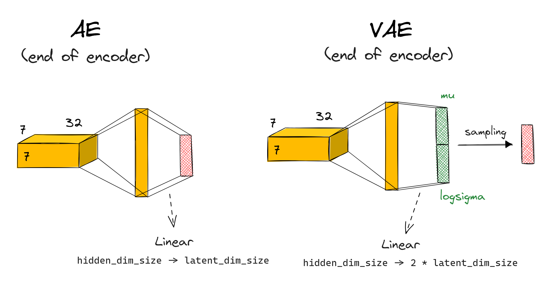
Probabilistic encoder
Rather than your encode outputting a latent vector $\boldsymbol{z}$, it should output a mean $\mu$ and standard deviation $\sigma$; both vectors of dimension latent_dim_size. We then sample our latent vector $\boldsymbol{z}$ using $z_i = \mu_i + \sigma_i \cdot \epsilon_i$. Note that this is equivalent to $z = \mu + \Sigma \epsilon$ as shown in the diagram above, but where we assume $\Sigma$ is a diagonal matrix (i.e. the auxiliary random variables $\epsilon$ which we're sampling are independent). This is the most common approach taken in situations like these.
Note - we actually calculate mu and logsigma rather than mu and sigma - we get sigma = logsigma.exp() from this. This is a more numerically stable method.
How exactly should this work in your model's architecture? You can replace the final linear layer (which previously just gave you the latent vector) with two linear layers returning mu and logsigma, then you calculate z from these (and from a randomly sampled epsilon). If you want, you can combine the two linear layers into one linear layer with out_channels=2*latent_dim_size, then rearrange to split this up into mu and logsigma (this is what we do in the solution, and in the diagram below).
You should also return the parameters mu and logsigma in your VAE's forward function, as well as the final output - the reasons for this will become clear below.
Exercise - build your VAE
```yaml Difficulty: 🔴🔴🔴⚪⚪ Importance: 🔵🔵🔵🔵⚪
You should spend up to 15-25 minutes on this exercise. ```
Build your VAE. It should be identical to the autoencoder you built above, except for the changes made at the end of the encoder (outputting mean and std rather than a single latent vector; this latent vector needs to get generated via the reparameterisation trick).
For consistency with code that will come later, we recommend having your model.encoder output be of shape (2, batch_size, latent_dim_size), where output[0] are the mean vectors $\mu$ and output[1] are the log standard deviation vectors $\log \sigma$. The tests below will check this.
We've also given you a sample_latent_vector method - this should return the output of your encoder, but in the form of sampled latent vectors $\mu$ and $\sigma$ rather than the deterministic output model.encoder(x) of shape (2, batch_size, latent_dim_size). This will be a useful method for later (and you can use it in your implementation of forward).
class VAE(nn.Module):
    encoder: nn.Module
    decoder: nn.Module

    def __init__(self, latent_dim_size: int, hidden_dim_size: int):
        super().__init__()
        self.encoder = ...
        self.decoder = ...

    def sample_latent_vector(self, x: Tensor) -> tuple[Tensor, Tensor, Tensor]:
        """
        Passes `x` through the encoder, returns tuple of (sampled latent vector, mean, log std dev).
        This function can be used in `forward`, but also used on its own to generate samples for
        evaluation.
        """
        raise NotImplementedError()

    def forward(self, x: Tensor) -> tuple[Tensor, Tensor, Tensor]:
        """
        Passes `x` through the encoder and decoder. Returns the reconstructed input, as well as mu
        and logsigma.
        """
        raise NotImplementedError()


tests.test_vae(VAE)
Solution
class VAE(nn.Module):
    encoder: nn.Module
    decoder: nn.Module
def __init__(self, latent_dim_size: int, hidden_dim_size: int):
        super().__init__()
        self.latent_dim_size = latent_dim_size
        self.hidden_dim_size = hidden_dim_size
        self.encoder = Sequential(
            Conv2d(1, 16, 4, stride=2, padding=1),
            ReLU(),
            Conv2d(16, 32, 4, stride=2, padding=1),
            ReLU(),
            Rearrange("b c h w -> b (c h w)"),
            Linear(7  7  32, hidden_dim_size),
            ReLU(),
            Linear(hidden_dim_size, latent_dim_size  2),
            Rearrange(
                "b (n latent_dim) -> n b latent_dim", n=2
            ),  # makes it easier to separate mu and sigma
        )
        self.decoder = nn.Sequential(
            Linear(latent_dim_size, hidden_dim_size),
            ReLU(),
            Linear(hidden_dim_size, 7  7  32),
            ReLU(),
            Rearrange("b (c h w) -> b c h w", c=32, h=7, w=7),
            ConvTranspose2d(32, 16, 4, stride=2, padding=1),
            ReLU(),
            ConvTranspose2d(16, 1, 4, stride=2, padding=1),
        )
def sample_latent_vector(self, x: Tensor) -> tuple[Tensor, Tensor, Tensor]:
        """
        Passes x through the encoder, returns tuple of (sampled latent vector, mean, log std dev).
        This function can be used in forward, but also used on its own to generate samples for
        evaluation.
        """
        mu, logsigma = self.encoder(x)
        sigma = t.exp(logsigma)
        z = mu + sigma  t.randn_like(sigma)
        return z, mu, logsigma
def forward(self, x: Tensor) -> tuple[Tensor, Tensor, Tensor]:
        """
        Passes x through the encoder and decoder. Returns the reconstructed input, as well as mu
        and logsigma.
        """
        z, mu, logsigma = self.sample_latent_vector(x)
        x_prime = self.decoder(z)
        return x_prime, mu, logsigma
You can also do the previous thing (compare your architecture to the solution), but this might be less informative if your model doesn't implement the 2-variables approach in the same way as the solution does.
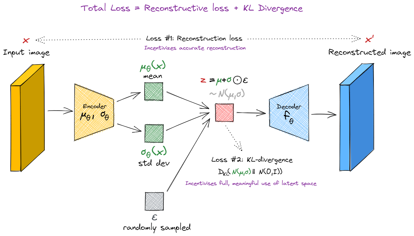
New loss function
We're no longer calculating loss simply as the reconstruction error between the original input $\boldsymbol{x}$ and our decoder's output $\boldsymbol{x}'$. Instead, we have a new loss function. For a fixed input $\boldsymbol{x}$, our loss is:
The first term is just the regular reconstruction loss we used for our autoencoder. The second term is the KL divergence between the generator's output distribution and the standard normal distribution, and it's designed to penalize the generator for producing latent vectors which are far from the standard normal distribution.
There is a much deeper way to understand this loss function, which also connects to intuitions around diffusion models and other more complicated generative models. For more on this, see the section at the end. For now, we'll move on to the practicalities of implementing this loss function.
The KL divergence of these two distributions has a closed form expression, which is given by:
This is why it was important to output mu and logsigma in our forward functions, so we could compute this expression! (It's easier to use logsigma than sigma when evaluating the expression above, for stability reasons).
We won't ask you to derive this formula, because it requires understanding of differential entropy which is a topic we don't need to get into here. However, it is worth doing some sanity checks, e.g. plot some graphs and convince yourself that this expression is larger as $\mu$ is further away from 0, or $\sigma$ is further away from 1.
(Note that we want our loss term to be a single number. When we calculate the KL divergence, we'll get a vector of latent_dim-many KL divergences between the $\mu$ and $\sigma$ of each of our normal distributions. To get our final KL loss penalty, we'll take the mean over this vector.)
Derivation of KL divergence result
If you'd like a derivation, you can find one [here](https://statproofbook.github.io/P/norm-kl), where a slightly more general form of the KL divergence between two normal distributions is derived. Our result is a special case of this, for $\mu_2 = 0$, $\sigma_2^2 = 1$. In this derivation, they use $\langle \cdot \rangle_{p(x)}$ to denote the expectation of a function under the distribution $p$, i.e. $\langle f(x) \rangle_{p(x)} = \mathbb{E}_{p} [ f(x) ] = \int_{\mathcal{X}} p(x) f(x) \; dx$. A more general result for multi-variate normal distributions with different means and covariances can be found [here](https://mr-easy.github.io/2020-04-16-kl-divergence-between-2-gaussian-distributions/).
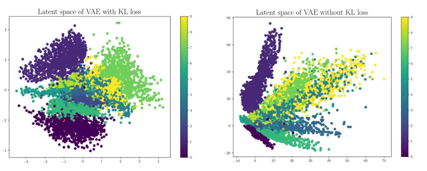
One can interpret this as the penalty term to make the latent space meaningful. If all the latent vectors $\boldsymbol{z}$ you generate have each component $z_i$ normally distributed with mean 0, variance 1 (and we know they're independent because our $\epsilon_i$ we used to generate them are independent), then there will be no gaps in your latent space where you produce weird-looking output (like we saw in our autoencoder plots from the previous section). You can try training your VAE without this term, and it might do okay at reproducing $\boldsymbol{x}$, but it will perform much worse when it comes time to use it for generation. Again, you can quantify this by encoding some input data and projecting it onto the first two dimensions. When you include this term you should expect to see a nice regular cloud surrounding the origin, but without this term you might see some irregular patterns or blind spots:
Once you've computed both of these loss functions, you should add them together and perform gradient descent on them.
Beta-VAEs
The Beta-VAE is a very simple extension of the VAE, with a different loss function: we multiply the KL Divergence term by a constant $\beta$. This helps us balance the two different loss terms. Here, we've given you the default value of $\beta = 0.1$ rather than using $\beta = 1$ (which is implicit when we use regular VAEs rather than beta-VAEs).
As a general comment on tuning hyperparameters like $\beta$, it's important to sweep over ranges of different values and know how to tell when one of them is dominating the model's behaviour. In this particular case, $\beta$ being too large means your model will too heavily prioritize having its latent vectors' distribution equal to the standard normal distribution, to the point where it might essentially lose all structure in the data and ignore accurate reconstruction. On the other hand, $\beta$ being too small means we just reduce to the autoencoder case where the model has no incentive to make meaningful use of the latent space. Weights and biases hyperparameter searches are a good tool for sweeping over ranges and testing the results, but they'll only work if you log the relevant data / output and know how to interpret it.
Exercise - write your VAE training loop
```yaml Difficulty: 🔴🔴🔴⚪⚪ Importance: 🔵🔵🔵⚪⚪
You should spend up to 15-30 minutes on this exercise. ```
You should write and run your training loop below. This will involve a lot of recycled code from the corresponding Autoencoder exercise - in fact, depending on how you implemented the train method before, you might literally be able to copy and paste that method here!
@dataclass
class VAEArgs(AutoencoderArgs):
    wandb_project: str | None = "day5-vae-mnist"
    beta_kl: float = 0.1


class VAETrainer:
    def __init__(self, args: VAEArgs):
        self.args = args
        self.trainset = get_dataset(args.dataset)
        self.trainloader = DataLoader(
            self.trainset, batch_size=args.batch_size, shuffle=True, num_workers=8
        )
        self.model = VAE(
            latent_dim_size=args.latent_dim_size,
            hidden_dim_size=args.hidden_dim_size,
        ).to(device)
        self.optimizer = t.optim.Adam(self.model.parameters(), lr=args.lr, betas=args.betas)

    def training_step(self, img: Tensor):
        """
        Performs a training step on the batch of images in `img`. Returns the loss. Logs to wandb
        if enabled.
        """
        raise NotImplementedError()

    @t.inference_mode()
    def log_samples(self) -> None:
        """
        Evaluates model on holdout data, either logging to wandb or displaying output inline.
        """
        assert self.step > 0, (
            "First call should come after a training step. Remember to increment `self.step`."
        )
        output = self.model(HOLDOUT_DATA)[0]
        if self.args.use_wandb:
            output = (output - output.min()) / (output.max() - output.min())  # Normalize to [0, 1]
            output = (output * 255).to(dtype=t.uint8)  # Convert to uint8 for logging
            wandb.log(
                {"images": [wandb.Image(arr) for arr in output.cpu().numpy()]}, step=self.step
            )
        else:
            display_data(t.concat([HOLDOUT_DATA, output]), nrows=2, title="VAE reconstructions")

    def train(self) -> VAE:
        """Performs a full training run."""
        self.step = 0
        if self.args.use_wandb:
            wandb.init(project=self.args.wandb_project, name=self.args.wandb_name)
            wandb.watch(self.model)

        # YOUR CODE HERE - iterate over epochs, and train your model

        if self.args.use_wandb:
            wandb.finish()

        return self.model


args = VAEArgs(latent_dim_size=5, hidden_dim_size=100, use_wandb=True)
trainer = VAETrainer(args)
vae = trainer.train()
Solution
@dataclass
class VAEArgs(AutoencoderArgs):
    wandb_project: str | None = "day5-vae-mnist"
    beta_kl: float = 0.1
class VAETrainer:
    def __init__(self, args: VAEArgs):
        self.args = args
        self.trainset = get_dataset(args.dataset)
        self.trainloader = DataLoader(
            self.trainset, batch_size=args.batch_size, shuffle=True, num_workers=8
        )
        self.model = VAE(
            latent_dim_size=args.latent_dim_size,
            hidden_dim_size=args.hidden_dim_size,
        ).to(device)
        self.optimizer = t.optim.Adam(self.model.parameters(), lr=args.lr, betas=args.betas)
def training_step(self, img: Tensor):
        """
        Performs a training step on the batch of images in img. Returns the loss. Logs to wandb
        if enabled.
        """
        # Get the different loss components, as well as the total loss
        img = img.to(device)
        img_reconstructed, mu, logsigma = self.model(img)
        reconstruction_loss = nn.MSELoss()(img, img_reconstructed)
        kl_div_loss = (
            0.5 * (mu**2 + t.exp(2  logsigma) - 1) - logsigma
        ).mean()  self.args.beta_kl
        loss = reconstruction_loss + kl_div_loss
# Backprop on the loss, and step with optimizers
        loss.backward()
        self.optimizer.step()
        self.optimizer.zero_grad()
# Log various values, and also increment self.step
        if self.args.use_wandb:
            wandb.log(
                dict(
                    reconstruction_loss=reconstruction_loss.item(),
                    kl_div_loss=kl_div_loss.item(),
                    mean=mu.mean(),
                    std=t.exp(logsigma).mean(),
                    total_loss=loss.item(),
                ),
                step=self.step,
            )
        return loss
@t.inference_mode()
    def log_samples(self) -> None:
        """
        Evaluates model on holdout data, either logging to wandb or displaying output inline.
        """
        assert self.step > 0, (
            "First call should come after a training step. Remember to increment self.step."
        )
        output = self.model(HOLDOUT_DATA)[0]
        if self.args.use_wandb:
            output = (output - output.min()) / (output.max() - output.min())  # Normalize to [0, 1]
            output = (output * 255).to(dtype=t.uint8)  # Convert to uint8 for logging
            wandb.log(
                {"images": [wandb.Image(arr) for arr in output.cpu().numpy()]}, step=self.step
            )
        else:
            display_data(t.concat([HOLDOUT_DATA, output]), nrows=2, title="VAE reconstructions")
def train(self) -> VAE:
        """Performs a full training run."""
        self.step = 0
        if self.args.use_wandb:
            wandb.init(project=self.args.wandb_project, name=self.args.wandb_name)
            wandb.watch(self.model)
for epoch in range(self.args.epochs):
            # Iterate over training data, performing a training step for each batch
            progress_bar = tqdm(self.trainloader, total=int(len(self.trainloader)), ascii=True)
            for img, label in progress_bar:  # remember that label is not used
                img = img.to(device)
                loss = self.training_step(img)
                self.step += 1
                progress_bar.set_description(f"{epoch=:02d}, {loss=:.4f}, batches={self.step:05d}")
                if self.step % self.args.log_every_n_steps == 0:
                    self.log_samples()
if self.args.use_wandb:
            wandb.finish()
return self.model
You might be disappointed when comparing your VAE's reconstruction to the autoencoder, since it's likely to be worse. However, remember that the focus of VAEs is in better generation, not reconstruction. To test it's generation, let's produce some plots of latent space like we did for the autoencoder.
First, we'll visualize the latent space:
grid_latent = create_grid_of_latents(vae, interpolation_range=(-1, 1))
output = vae.decoder(grid_latent)
utils.visualise_output(output, grid_latent, title="VAE latent space visualization")
Click to see the expected output
which should look a lot better! The vast majority of images in this region should be recognisable digits. In this case, starting from the top-left and going clockwise, we can see 0s, 6s, 5s, 1s, 9s and 8s. Even the less recognisable regions seem like they're just interpolations between digits which are recognisable (which is something we should expect to happen given our VAE's output is continuous).
Now for the scatter plot to visualize our input space:
small_dataset = Subset(get_dataset("MNIST"), indices=range(0, 5000))
imgs = t.stack([img for img, label in small_dataset]).to(device)
labels = t.tensor([label for img, label in small_dataset]).to(device).int()

# We're getting the mean vector, which is the [0]-indexed output of the encoder
latent_vectors = vae.encoder(imgs)[0, :, :2]
holdout_latent_vectors = vae.encoder(HOLDOUT_DATA)[0, :, :2]

utils.visualise_input(latent_vectors, labels, holdout_latent_vectors, HOLDOUT_DATA)
Click to see the expected output
The range of the distribution looks much more like a standard normal distribution (most points are in [-2, 2] whereas in the previous plot the range was closer to [-10, 10]). There are also no longer any large gaps in the latent space that you wouldn't find in the corresponding standard normal distribution.
To emphasize - don't be disheartened if your reconstructions of the original MNIST images don't look as faithful for your VAE than they did for your encoder. Remember the goal of these architectures isn't to reconstruct images faithfully, it's to generate images from samples in the latent dimension. This is the basis on which you should compare your models to each other.
A deeper dive into the maths of VAEs
If you're happy with the loss function as described in the section above, then you can move on from here. If you'd like to take a deeper dive into the mathematical justifications of this loss function, you can read the following content. I'd consider it pretty essential in laying the groundwork for understanding diffusion models, and most kinds of generative image models (which we might dip into later in this course).
Note - this section is meant to paint more of an intuitive picture than deal with formal and rigorous mathematics, which is why we'll play fairly fast and loose with things like limit theorems and whether we can swap around integrals and expected values. This can be formalized further, but we'll leave that for other textbooks.
Firstly, let's ignore the encoder, and suppose we're just starting from a latent vector $\boldsymbol{z} \sim p(z) = N(0, I)$. We can parameterize a probabilistic decoder as $p_\theta(\boldsymbol{x} \mid \boldsymbol{z})$, i.e. a way of mapping from latent vectors $z$ to a distribution over images $\boldsymbol{x}$. To use it as a decoder, we just sample a latent vector then sample from the resulting probability distribution our decoder gives us. Imagine this as a factory line: the latent vector $\boldsymbol{z}$ is some kind of compressed blueprint for our image, and our decoder is a way of reconstructing images from this information.
On this factory line, the probability of producing any given image $\boldsymbol{x}$ can be found from integrating over the possible latent vectors $\boldsymbol{z}$ which could have produced it:
Unfortunately, it's not that easy. Evaluating this integral would be computationally intractible, because we would have to sample over all possible values for the latent vectors $\boldsymbol{z}$:
This is where our encoder function $q_\phi(\boldsymbol{z} \mid \boldsymbol{x})$ comes in! It helps concentrate our guess for $\boldsymbol{z}$ for any given $\boldsymbol{x}$, essentially telling us which latent vectors were likely to have produced the image $\boldsymbol{x}$. We can now replace our original integral with the following:
We now introduce an important quantity, called the ELBO, or evidence lower-bound. It is defined as the value inside the expectation in the expression above, but using log instead.
It turns out that by looking at log probs rather than probabilities, we can now rewrite the ELBO as something which looks a lot like our VAE loss function! $p_\theta(\boldsymbol{x} \mid \boldsymbol{z})$ is our decoder, $q_\phi(\boldsymbol{z} \mid \boldsymbol{x})$ is our encoder, and we train them jointly using gradient ascent on our estimate of the ELBO. For any given sample $x_i$, the value $\operatorname{ELBO}(x_i)$ is estimated by sampling a latent vector $z_i \sim q_\phi(\boldsymbol{z} \mid \boldsymbol{x_i})$, and then performing gradient ascent on the ELBO, which can be rewritten as:
- The first term is playing the role of reconstruction loss, since it's equivalent to the log probability that our image $x$ is perfectly reconstructed via the series of maps $\boldsymbol{x} \xrightarrow{\text{encoder}} \boldsymbol{z} \xrightarrow{\text{decoder}} \boldsymbol{x}$. If we had perfect reconstruction then this value would be zero (which is its maximum value).
- The second term is the KL divergence between $q_\phi(\boldsymbol{z} \mid \boldsymbol{x})$ and $p_{\theta}(\boldsymbol{z})$. The former is your own encoder's distribution of latent vectors which you may recall is $N(\mu(\boldsymbol{x}), \sigma(\boldsymbol{x})^2)$, and the latter was assumed to be the uniform distribution $N(0, I)$. This just reduces to our KL penalty term from earlier.
The decoder used in our VAE isn't actually probabilistic $p_\theta(\cdot \mid \boldsymbol{z})$, it's deterministic (i.e. it's a map from latent vector $\boldsymbol{z}$ to reconstructed input $\boldsymbol{x}'$). But we can pretend that the decoder output is actually the mean of a probability distribution, and we're choosing this mean as the value of our reconstruction $\boldsymbol{x}'$. The reconstruction loss term in the formula above will be smallest when this mean is close to the original value $\boldsymbol{x}$ (because then $p_\theta(\cdot \mid \boldsymbol{z})$ will be a probability distribution centered around $\boldsymbol{x}$). And it turns out that we can just replace this reconstruction loss with something that fulfils basically the same purpose (the $L_2$ penalty) - although we sometimes need to adjust these two terms (see $\beta$-VAEs above).
And that's the math of VAEs in a nutshell!
Bonus exercises
PCA
In the code earlier, we visualised our autoencoder / VAE output along the first two dimensions of the latent space. If each dimension is perfectly IID then we should expect this to get similar results to varying along any two arbitrarily chosen orthogonal directions. However, in practice you might find it an improvement to choose directions in a more principled way. One way to do this is to use principal component analysis (PCA). Can you write code to extract the PCA components from your model's latent space, and plot the data along these components?
Template (code for extracting PCA from the Autoencoder)
from sklearn.decomposition import PCA
@t.inference_mode()
def get_pca_components(
    model: Autoencoder,
    dataset: Dataset,
) -> tuple[Tensor, Tensor]:
    '''
    Gets the first 2 principal components in latent space, from the data.
    Returns:
        pca_vectors: shape (2, latent_dim_size)
            the first 2 principal component vectors in latent space
        principal_components: shape (batch_size, 2)
            components of data along the first 2 principal components
    '''
    # Unpack the (small) dataset into a single batch
    imgs = t.stack([batch[0] for batch in dataset]).to(device)
    labels = t.tensor([batch[1] for batch in dataset])
# Get the latent vectors
    latent_vectors = model.encoder(imgs.to(device)).cpu().numpy()
    if latent_vectors.ndim == 3: latent_vectors = latent_vectors[0] # useful for VAEs; see later
# Perform PCA, to get the principle component directions (& projections of data in these dirs)
    pca = PCA(n_components=2)
    principal_components = pca.fit_transform(latent_vectors)
    pca_vectors = pca.components_
    return (
        t.from_numpy(pca_vectors).float(),
        t.from_numpy(principal_components).float(),
    )
And then you can use this function in your visualise_output by replacing the code at the start with this:
pca_vectors, principal_components = get_pca_components(model, dataset)
# Constructing latent dim data by making two of the dimensions vary independently in the
# interpolation range.
x = t.linspace(interpolation_range, n_points)
grid_latent = t.stack([
    einops.repeat(x, "dim1 -> dim1 dim2", dim2=n_points),
    einops.repeat(x, "dim2 -> dim1 dim2", dim1=n_points),
], dim=-1)
# Map grid to the basis of the PCA components
grid_latent = grid_latent @ pca_vectors
Note that this will require adding dataset to the arguments of this function.
You can do something similar for the visualise_input function:
@t.inference_mode()
def visualise_input(
    model: Autoencoder,
    dataset: Dataset,
) -> None:
    '''
    Visualises (in the form of a scatter plot) the input data in the latent space, along the first
    two latent dims.
    '''
    # First get the model images' latent vectors, along first 2 dims
    imgs = t.stack([batch for batch, label in dataset]).to(device)
    latent_vectors = model.encoder(imgs)
    if latent_vectors.ndim == 3: latent_vectors = latent_vectors[0] # useful for VAEs later
    latent_vectors = latent_vectors[:, :2].cpu().numpy()
    labels = [str(label) for img, label in dataset]
# Make a dataframe for scatter (px.scatter is more convenient to use when supplied with a dataframe)
    df = pd.DataFrame({"dim1": latent_vectors[:, 0], "dim2": latent_vectors[:, 1], "label": labels})
    df = df.sort_values(by="label")
    fig = px.scatter(df, x="dim1", y="dim2", color="label")
    fig.update_layout(height=700, width=700, title="Scatter plot of latent space dims", legend_title="Digit")
    data_range = df["dim1"].max() - df["dim1"].min()
# Add images to the scatter plot (optional)
    output_on_data_to_plot = model.encoder(HOLDOUT_DATA.to(device))
    if output_on_data_to_plot.ndim == 3:
        output_on_data_to_plot = output_on_data_to_plot[0] # useful for VAEs later
    output_on_data_to_plot = output_on_data_to_plot[:, :2].cpu()
    data_translated = (HOLDOUT_DATA.cpu().numpy()  0.3081) + 0.1307
    data_translated = (255 * data_translated).astype(np.uint8).squeeze()
    for i in range(10):
        x, y = output_on_data_to_plot[i]
        fig.add_layout_image(
            source=Image.fromarray(data_translated[i]).convert("L"),
            xref="x", yref="y",
            x=x, y=y,
            xanchor="right", yanchor="top",
            sizex=data_range/15, sizey=data_range/15,
        )
    fig.show()
Beta-VAEs
Read the section on Beta-VAEs, if you haven't already. Can you choose a better value for $\beta$?
To decide on an appropriate $\beta$, you can look at the distribution of your latent vector. For instance, if your latent vector looks very different to the standard normal distribution when it's projected onto one of its components (e.g. maybe that component is very sharply spiked around some particular value), this is a sign that you need to use a larger parameter $\beta$. You can also just use hyperparameter searches to find an optimal $\beta$. See the paper which introduced Beta-VAEs for more ideas.
CelebA dataset
Try to build an autoencoder for the CelebA dataset. You shouldn't need to change the architecture much from your MNIST VAE. You should find the training much easier than with your GAN (as discussed yesterday, GANs are notoriously unstable when it comes to training). Can you get better results than you did for your GAN?
Hierarchical VAEs
Hierarchical VAEs are ones which stack multiple layers of parameter-learning and latent-vector-sampling, rather than just doing this once. Read the section of this paper for a more thorough description.
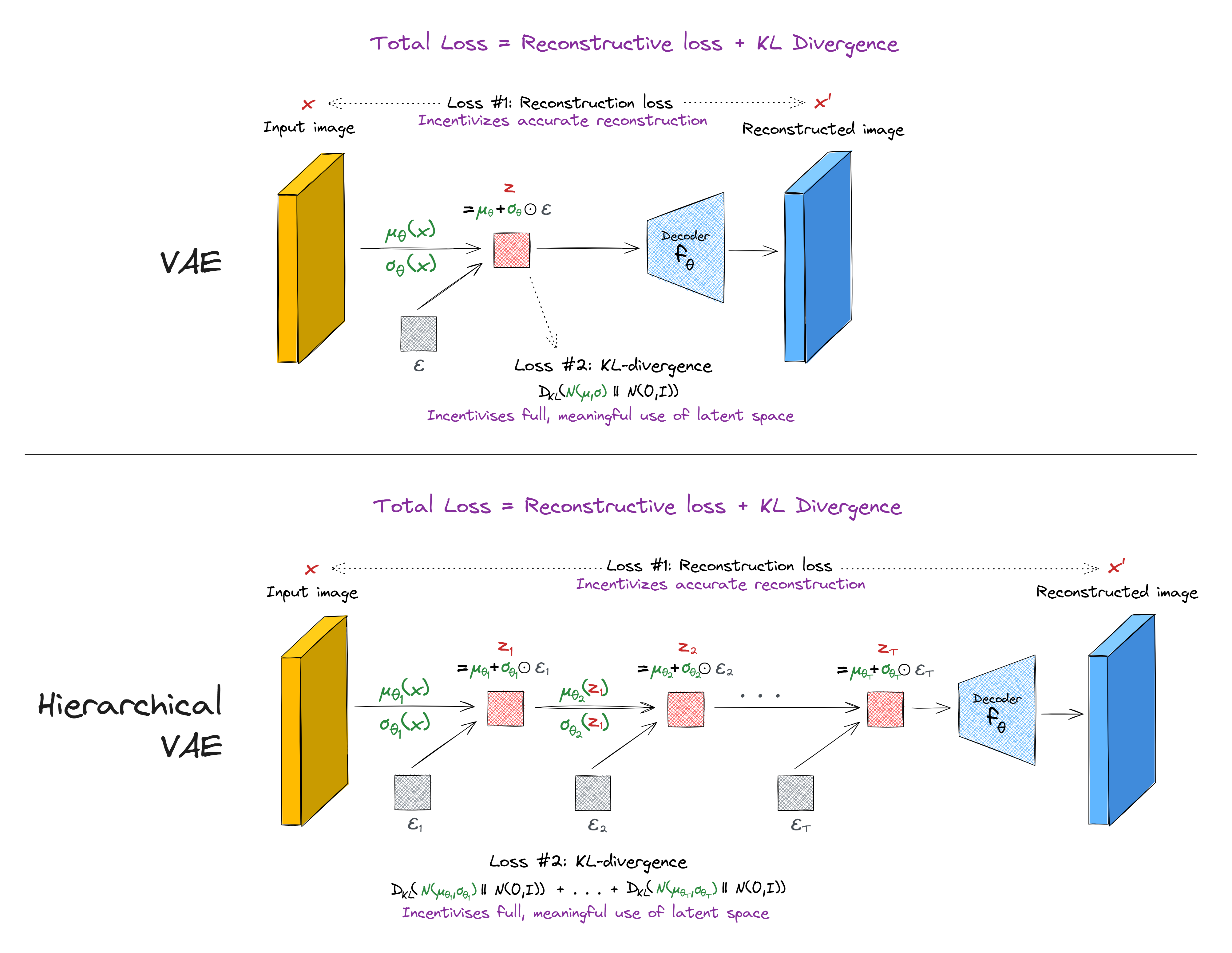
(Note - the KL divergence loss used in HVAEs can sometimes be more complicated than the one presented in this diagram, if you want to implement conditional dependencies between the different layers. However, this isn't necessary for the basic HVAE architecture.)
Try to implement your own hierarchical VAE.
Note - when you get to the material on diffusion models later in the course, you might want to return here, because understanding HVAEs can be a useful step to understanding diffusion models. In fact diffusion models can almost be thought of as a special type of HVAE.
Denoising and sparse autoencoders
The reading material on VAEs talks about denoising and sparse autoencoders. Try changing the architecture of your autoencoder (not your VAE) to test out one of these two techniques. Do does your decoder output change? How about your encoder scatter plot?
Note - sparse autoencoders will play an important role in some later sections of this course (when we study superposition in mechanistic interpretability).
If you're mathematically confident and feeling like a challenge, you can also try to implement contractive autoencoders!