1️⃣ Introduction to backprop
Learning Objectives
- Understand what a computational graph is, and how it can be used to calculate gradients.
- Start to implement backwards versions of some basic functions.
Reading
Computing Gradients with Backpropagation
This section will briefly review the backpropagation algorithm, but focus mainly on the concrete implementation in software.
To train a neural network, we want to know how the loss would change if we slightly adjust one of the learnable parameters.
One obvious and straightforward way to do this would be just to add a small value to the parameter, and run the forward pass again. This is called finite differences, and the main issue is we need to run a forward pass for every single parameter that we want to adjust. This method is infeasible for large networks, but it's important to know as a way of sanity checking other methods.
A second obvious way is to write out the function for the entire network, and then symbolically take the gradient to obtain a symbolic expression for the gradient. This also works and is another thing to check against, but the expression gets quite complicated.
Suppose that you have some computational graph, and you want to determine the derivative of the some scalar loss L with respect to NumPy arrays a, b, and c:
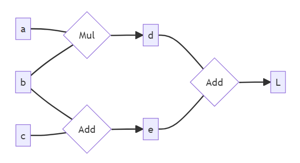
This graph corresponds to the following Python:
d = a * b
e = b + c
L = d + e
The goal of our system is that users can write ordinary looking Python code like this and have all the book-keeping needed to perform backpropagation happen behind the scenes. To do this, we're going to wrap each array and each function in special objects from our library that do the usual thing plus build up this graph structure that we need.
Backward Functions
We've drawn our computation graph from left to right and the arrows pointing to the right, so that in the forward pass, boxes to the right depend on boxes to the left. In the backwards pass, the opposite is true: the gradient of boxes on the left depends on the gradient of boxes on the right.
If we want to compute the derivative of $L$ wrt all other variables (as was described in the reading), we should traverse the graph from right to left. Each time we encounter an instance of function application, we can use the chain rule from calculus to proceed one step further to the left. For example, if we have $d = a \times b$, then:
Suppose we are working from right to left, trying to calculate $\frac{dL}{da}$. If we already know the values of the variables $a$, $b$ and $d$, as well as the value of $\frac{dL}{dd}$, then we can use the following function to find $\frac{dL}{da}$:
and we can do something similar when trying to calculate $\frac{dL}{db}$.
In other words, we can take the "forward function" $(a, b) \to a \cdot b$, and for each of its parameters, we can define an associated "backwards function" which tells us how to compute the gradient wrt this argument using only known quantities as inputs.
Ignoring issues of unbroadcasting (which we'll cover later), we could write the backward with respect to the first argument as:
def multiply_back(grad_out, out, a, b):
    '''
    Inputs:
        grad_out = dL/d(out)
        out = a * b

    Returns:
        dL/da
    '''
    return grad_out * b
where grad_out is the gradient of the loss of the function with respect to the output (i.e. $\frac{dL}{dd}$), out is the output of the function (i.e. $d$), and a and b are our inputs.
Topological Ordering
When we're actually doing backprop, how do we guarantee that we'll always know the value of our backwards functions' inputs? For instance, in the example above we couldn't have computed $\frac{dL}{da}$ without first knowing $\frac{dL}{dd}$.
The answer is that we sort all our nodes using an algorithm called topological sorting, and then do our computations in this order. After each computation, we store the gradients in our nodes for use in subsequent calculations.
When described in terms of the diagram above, topological sort can be thought of as an ordering of nodes from right to left. Crucially, this sorting has the following property: if there is a directed path in the computational graph going from node x to node y, then x must follow y in the sorting.
There are many ways of proving that a cycle-free directed graph contains a topological ordering. You can try and prove this for yourself, or click on the expander below to reveal the outline of a simple proof.
Click to reveal proof
We can prove by induction on the number of nodes $N$.
If $N=1$, the problem is trivial.
If $N>1$, then pick any node, and follow the arrows until you reach a node with no directed arrows going out of it. Such a node must exist, or else you would be following the arrows forever, and you'd eventually return to a node you previously visited, but this would be a cycle, which is a contradiction. Once you've found this "root node", you can put it first in your topological ordering, then remove it from the graph and apply the topological sort on the subgraph created by removing this node. By induction, your topological sorting algorithm on this smaller graph should return a valid ordering. If you append the root node to the start of this ordering, you have a topological ordering for the whole graph.
A quick note on some potentially confusing terminology. We will refer to the "end node" as the root node, and the "starting nodes" as leaf nodes. For instance, in the diagram at the top of the section, the left nodes a, b and c are the leaf nodes, and L is the root node. This might seem odd given it makes the leaf nodes come before the root nodes, but the reason is as follows: when we're doing the backpropagation algorithm, we start at L and work our way back through the graph. So, by our notation, we start at the root node and work our way out to the leaves.
Another important piece of terminology here is parent node. This means the same thing as it does in most other contexts - the parents of node x are all the nodes y with connections y -> x (so in the diagram, L's parents are d and e).
Question - can you think of a reason it might be important for a node to store a list of all of its parent nodes?
During backprop, we're moving from right to left in the diagram. If a node doesn't store its parent, then there will be no way to get access to that parent node during backprop, so we can't propagate gradients to it.
The very first node in our topological sort will be $L$, the root node.
Backpropagation
After all this setup, the backpropagation mechanism becomes pretty straightforward. We sort the nodes topologically, then we iterate over them and call each backward function exactly once in order to accumulate the gradients at each node.
It's important that the grads be accumulated instead of overwritten in a case like value $b$ which has two outgoing edges, since $\frac{dL}{db}$ will then be the sum of two terms. Since addition is commutative it doesn't matter whether we backward() the Mul or the Add that depend on $b$ first.
During backpropagation, for each forward function in our computational graph we need to find the partial derivative of the output with respect to each of its inputs. Each partial is then multiplied by the gradient of the loss with respect to the forward functions output (grad_out) to find the gradient of the loss with respect to each input. We'll handle these calculations using backward functions.
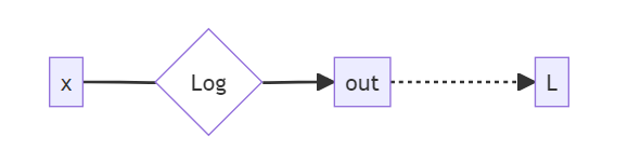
Backward function of log
First, we'll write the backward function for x -> out = log(x). This should be a function which, when fed the values x, out, grad_out = dL/d(out) returns the value of dL/dx just from this particular computational path.
Note - it might seem strange at first why we need x and out to be inputs, out can be calculated directly from x. The answer is that sometimes it is computationally cheaper to express the derivative in terms of out than in terms of x.
Question - can you think of an example function where it would be computationally cheaper to use 'out' than to use 'x'?
The most obvious answer is the exponential function, out = e ^ x. Here, the gradient d(out)/dx is equal to out. We'll see this when we implement a backward version of torch.exp later today.
Exercise - implement log_back
You should fill in this function below. Don't worry about division by zero or other edge cases - the goal here is just to see how the pieces of the system fit together.
This should just be a short, one-line function.
def log_back(grad_out: Arr, out: Arr, x: Arr) -> Arr:
    """Backwards function for f(x) = log(x)

    grad_out: Gradient of some loss wrt out
    out: the output of np.log(x).
    x: the input of np.log.

    Return: gradient of the given loss wrt x
    """
    raise NotImplementedError()


tests.test_log_back(log_back)
Help - I'm not sure what the output of this backward function for log should be.
By the chain rule, we have:
(Note - technically, $\frac{d(\text{out})}{dx}$ is a tensor containing the derivatives of each element of $\text{out}$ with respect to each element of $x$, and we should matrix multiply when we use the chain rule. However, since $\text{out} = \log x$ is an elementwise function of $x$, our application of the chain rule here will also be an elementwise multiplication: $\frac{dL}{dx_{ij}} = \frac{dL}{d(\text{out}_{ij})} \cdot \frac{d(\text{out}_{ij})}{dx_{ij}}$. When we get to things like matrix multiplication later, we'll have to be a bit more careful!)
Help - I get ImportError: numpy.core.multiarray failed to import
This is an annoying colab-related error which I haven't been able to find a satisfying fix for. The setup code at the top of this notebook should have installed a version of numpy which works, although you'll have to click "Restart Runtime" (from the Runtime menu) to make this work. Make sure you don't re-run the cell with pip installs.
If this still doesn't work, please flag it in the Slack channel errata.
Solution
def log_back(grad_out: Arr, out: Arr, x: Arr) -> Arr:
    """Backwards function for f(x) = log(x)

    grad_out: Gradient of some loss wrt out
    out: the output of np.log(x).
    x: the input of np.log.

    Return: gradient of the given loss wrt x
    """
    return grad_out / x
Backward functions of two tensors
Now we'll implement backward functions for multiple tensors. From this point onwards, we'll be working with vector-valued derivatives, i.e. terms like $\frac{\partial x}{\partial y}$ where $y$ (and possibly $x$) are tensors. To recap what this notation means - these terms are tensors where each value is the scalar derivative of one of the elements of $x$ wrt one of the elements of $y$. For example:
- If $x$ is a scalar and $y$ is a tensor with shape
(3, 4), then $\frac{\partial x}{\partial y}$ is a tensor with shape(3, 4)where the[i, j]-th element is $\frac{\partial x}{\partial y[i, j]}$, i.e. the derivative of $x$ wrt a particular element of $y$. - If $x$ is a length-5 vector and $y$ is a tensor with shape
(3, 4)then $\frac{\partial x}{\partial y}$ is a tensor with shape(5, 3, 4)where the[i, j, k]-th element is $\frac{\partial x[i]}{\partial y[j, k]}$.
Broadcasting
Before we go through the next exercises, we'll need to address one important topic in tensor operations - broadcasting. We've discussed it in earlier exercises, but we're reviewing it here because it's very important for backprop. If you're comfortable with the topic, feel free to jump forwards to the section "Why do we need broadcasting for backprop?".
Both NumPy and PyTorch have the same rules for broadcasting. When two tensors are involved in an elementwise operation, NumPy/PyTorch tries to broadcast them (i.e. copying them along dimensions) so that they both have the same shape. The rules of broadcasting are as follows:
- You can prepend dummy dimensions (of size 1) to the start of a tensor until both have the same number of dimensions
- After this point, if some dimension has size 1 in one of the tensors, it can be repeated until it matches the size of the corresponding dimension in the other tensor
To give a simple example - suppose we have a 2D batch of data, of shape data.shape = (N, k) (i.e. we have N separate datapoints, each being a vector of length k). Suppose we want to add a vector vec of length k to each datapoint. This is a valid operation, because when we try and add these two objects together:
vecgets prepended with a dummy dimension so it has shape(1, k)and both are 2Dvecgets repeated along the first dimension so it has shape(N, k), matching the shape ofdata
Then, our output has shape (N, k), and elements output[i, j] = data[i, j] + vec[j].
Broadcasting can be a very easy place to make mistakes, because it's easy to lose track of the exact shape of your tensors involved. As a warm-up exercise, below are some examples of broadcasting. Can you figure out which are valid, and which will raise errors?
x = np.ones((3, 1, 5))
y = np.ones((1, 4, 5))

z = x + y
Answer
This is valid, because the 0th dimension of y and the 1st dimension of x can both be copied so that x and y have the same shape: (3, 4, 5). The resulting array z will also have shape (3, 4, 5).
This example illustrates an important point - it's not always the case that one of the tensors is strictly smaller and the other is strictly bigger. Sometimes, both tensors will get expanded.
x = np.ones((8, 2, 6))
y = np.ones((8, 2))

z = x + y
Answer
This is not valid. We first need to expand y by appending a dimension to the front, and the last two dimensions of x are (2, 6), which won't broadcast with y's (8, 2).
x = np.ones((8, 2, 6))
y = np.ones((2, 6))

z = x + y
Answer
This is valid. Once NumPy expands y by appending a single dimension to the front, it can then be broadcast with x.
x = np.ones((10, 20, 30))
y = np.ones((20, 1))

z = x + y
Answer
This is valid. Once NumPy expands y by appending a single dimension to the front, it can then be broadcast with x (this will involve copying along the first and last dimensions).
x = np.ones((4, 1))
y = np.ones((4,))

z = x + y
Answer
This is valid. Numpy will expand the second one to (1, 4) then broadcast them both to (4, 4).
Although this won't raise an error, it's very possible that this isn't what the person adding these two arrays intended. A common source of mistakes is when you add 2 tensors thinking they're the same shape, but one actually has a dummy dimension you forgot about. Sadly this is something you'll just have to be vigilant for (e.g. adding assert statements where necessary, or making sure you aren't combining too many different tensor operations in a single line), because PyTorch doesn't have built-in ways of statically checking your tensor shapes.
Why do we need broadcasting for backprop?
Often, operations like out = f(x, y) involve an implicit broadcasting step. For example, if out = x + y with x.shape = (4,) and y.shape = (3, 4), then really our operation has 2 steps:
- Broadcast
xto a broadcasted versionx_bwhich has the shape ofy, i.e. copy it along the zeroth dimension to have shape(3, 4), - Define
out = x_b + y, which is an operation that doesn't involve broadcasting.
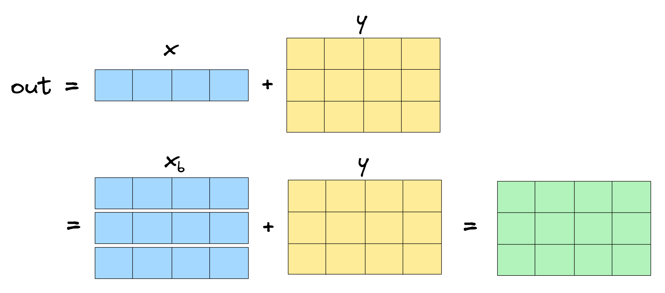
How can we go from the gradient dL/d(x_b) (which might be easy to compute given it involves no broadcasting) to the gradient of dL/dx? The answer is that we take dL/d(x_b) and sum it over the dimensions along which x was broadcasted to get dL/dx.
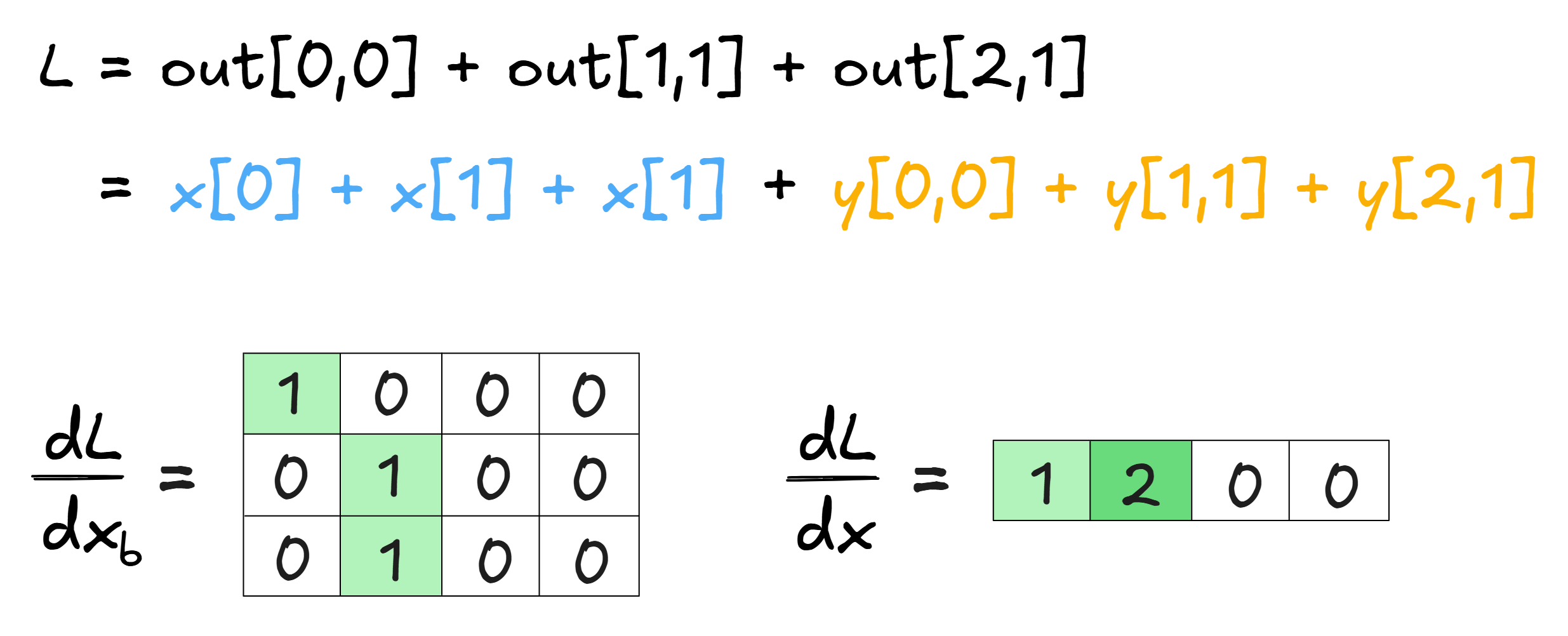
For the mathematically inclined this can be proved fairly easily (we provide a sketch of the proof below). But let's focus on the intuition here. When we copy x along axes to create x_b, we're essentially creating multiple pathways for each element of x to affect the final loss: one path for each time the element of x was copied. So when we change some element of x, this causes a first-order change in the loss from all of these different pathways, and we have to sum these changes to get the total first-order change (i.e. the derivative). For example:
Summary
If we know $\frac{\partial L}{\partial (\mathbf{out})}$, and want to know $\frac{\partial L}{\partial \mathbf{x}}$ (where $x$ was broadcasted to produce $\text{out}$) then there are two steps:
- Compute $\frac{\partial L}{\partial \mathbf{x_b}}$ in the standard way, i.e. using one of your backward functions (assuming no broadcasting happened).
- Unbroadcast $\frac{\partial L}{\partial \mathbf{x_b}}$, by summing it over the dimensions along which $\mathbf{x}$ was broadcasted.
Mathematical derivation (sketch)
We start with:
using the chain rule. Next, we can use the fact that $\frac{\partial x_b[i_1, i_2, ...]}{\partial x[j_1, j_2, ...]}$ equals 0 everywhere except the indices where $x$ was broadcasted to produce $x_b$, where it equals 1. Therefore, this sum over indices $i_1, i_2, ...$ is equivalent to just summing $\frac{\partial L}{\partial x_b[i_1, i_2, ...]}$ over the repeated elements of $x$.
We used the term "unbroadcast" because the way that our tensor's shape changes will be the reverse of how it changed during broadcasting. If x was broadcasted from (4,) -> (3, 4), then unbroadcasting will have to take a tensor of shape (3, 4) and sum over it to return a tensor of shape (4,). Similarly, if x was broadcasted from (1, 4) -> (3, 4), then we need to sum over the zeroth dimension, but leave it as a 2D tensor with a leading dummy dimension of size 1.
Exercise - implement unbroadcast
The unbroadcast function below should take any value like $\frac{\partial L}{\partial x_b}$ and return $\frac{\partial L}{\partial x}$ (where the arguments original and broadcasted represent $x$ and $x_b$ respectively). In the same way that broadcasting original to the shape of broadcasted can be described as a 2-step process:
- Extend dummy dimensions (size 1) of
originalto match the last dimensions ofbroadcasted, - Prepend dimensions to
originaluntil it has the same ndims asbroadcasted,
the unbroadcasting process is the same process in reverse:
- Sum over prepended dimensions of
broadcasteduntil it has the same ndims asoriginal, - Now they have the same ndims, sum over dimensions of
broadcastedwhereoriginalhad size 1.
For example, if original.shape = (3, 1) and broadcasted.shape = (1, 2, 3, 4) then the broadcasting steps look like (3, 1) -> (3, 4) -> (1, 2, 3, 4) (copying along those dimensions at each step) and the unbroadcasting steps look like (1, 2, 3, 4) -> (3, 4) -> (3, 1) (summing over those dimensions at each step).
def unbroadcast(broadcasted: Arr, original: Arr) -> Arr:
    """
    Sum 'broadcasted' until it has the shape of 'original'.

    broadcasted: An array that was formerly of the same shape of 'original' and was expanded by
        broadcasting rules.
    """
    # YOUR CODE HERE: sum over `broadcasted` until it has the shape of `original`

    assert broadcasted.shape == original.shape
    return broadcasted


tests.test_unbroadcast(unbroadcast)
Solution
def unbroadcast(broadcasted: Arr, original: Arr) -> Arr:
    """
    Sum 'broadcasted' until it has the shape of 'original'.

    broadcasted: An array that was formerly of the same shape of 'original' and was expanded by
        broadcasting rules.
    """
    # Step 1: sum and remove prepended dims, so both arrays have same number of dims
    n_dims_to_sum = len(broadcasted.shape) - len(original.shape)
    broadcasted = broadcasted.sum(axis=tuple(range(n_dims_to_sum)))

    # Step 2: sum over dims which were originally 1 (but don't remove them)
    dims_to_sum = tuple([i for i, (o, b) in enumerate(zip(original.shape, broadcasted.shape)) if o == 1 and b > 1])
    broadcasted = broadcasted.sum(axis=dims_to_sum, keepdims=True)

    assert broadcasted.shape == original.shape
    return broadcasted
Backward Function for Elementwise Multiply
Functions that are differentiable with respect to more than one input tensor are straightforward given that we already know how to handle broadcasting.
- We're going to have two backwards functions, one for each input argument.
- If the input arguments were broadcasted together to create a larger output, the incoming
grad_outwill be of the larger common broadcasted shape and we need to make use ofunbroadcastfrom earlier to match the shape to the appropriate input argument. - We'll want our backward function to work when one of the inputs is a float (as opposed to a tensor). We won't need to calculate the grad_in with respect to floats, so we only need to consider when y is a float for
multiply_back0and when x is a float formultiply_back1.
Exercise - implement both multiply_back functions
Below, you should implement both multiply_back0 and multiply_back1.
You might be wondering why we need two different functions, rather than just having a single function to serve both purposes. This will become more important later on, once we deal with functions with more than one argument, which is not symmetric in its arguments. For instance, the derivative of $x / y$ wrt $x$ is not the same as the expression you get after differentiating this wrt $y$ then swapping the labels around.
The first part of each function has been provided for you (this makes sure that both inputs are arrays, since we want to support multiplication by floats or scalars).
def multiply_back0(grad_out: Arr, out: Arr, x: Arr, y: Arr | float) -> Arr:
    """Backwards function for x * y wrt argument 0 aka x."""
    if not isinstance(y, Arr):
        y = np.array(y)

    raise NotImplementedError()


def multiply_back1(grad_out: Arr, out: Arr, x: Arr | float, y: Arr) -> Arr:
    """Backwards function for x * y wrt argument 1 aka y."""
    if not isinstance(x, Arr):
        x = np.array(x)

    raise NotImplementedError()


tests.test_multiply_back(multiply_back0, multiply_back1)
tests.test_multiply_back_float(multiply_back0, multiply_back1)
Hint
Using the chain rule for scalar functions, we can find that:
An equivalent result* holds for vector-valued inputs:
where $\cdot$ is the elementwise multiplication operator, and $\mathbf{x}_b, \mathbf{y}_b$ are the broadcasted versions of the input tensors. This allows us to compute $\frac{\partial L}{\partial \mathbf{x}_b}$ based on the inputs to our multiply_back0 function. Can you use unbroadcast to finish the calculation?
*You can derive this result for yourself using the chain rule. Note that application of the chain rule here would require you to sum over the elements of the intermediate tensor $\mathbf{x}_b \cdot \mathbf{y}_b$, but we're working with elementwise operations so $\partial (\mathbf{x}_b \cdot \mathbf{y}_b)[i_1, i_2, ...] / \partial \mathbf{x}_b$ will have all elements zero except for one and the sum falls out, leaving us with the result above.
Solution (and explanation)
Based on the discussion in hint 1, we can conclude that the value $\partial L / \partial \mathbf{x}_b$ is equal to y_b * grad_out. Note that this is just equivalent to y * grad_out because y will be broadcasted to the shape of y_b when we multiply it with grad_out (since we know grad_out has the same shape as the broadcasted x * y tensor).
Now, we need to go from this broadcasted derivative to the shape of x, and we do this by applying unbroadcast, summing y * grad_out over dimensions so that it's the same shape as x - in other words, we return unbroadcast(y * grad_out, x).
The output of multiply_back1 is the same as multiply_back0, except the roles of x and y are reversed.
def multiply_back0(grad_out: Arr, out: Arr, x: Arr, y: Arr | float) -> Arr:
    """Backwards function for x * y wrt argument 0 aka x."""
    if not isinstance(y, Arr):
        y = np.array(y)

    return unbroadcast(y * grad_out, x)


def multiply_back1(grad_out: Arr, out: Arr, x: Arr | float, y: Arr) -> Arr:
    """Backwards function for x * y wrt argument 1 aka y."""
    if not isinstance(x, Arr):
        x = np.array(x)

    return unbroadcast(x * grad_out, y)
Now we'll use our backward functions to do backpropagation manually, for the following computational graph:
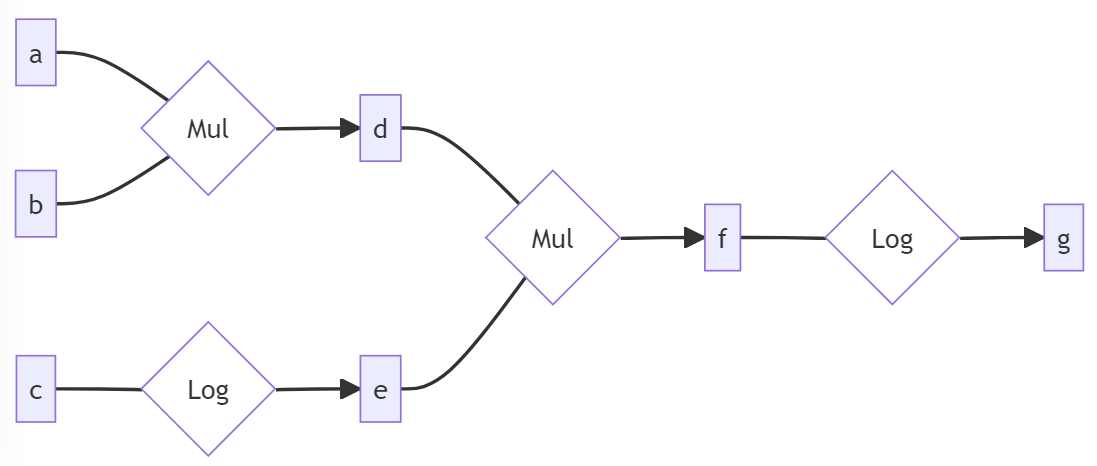
Exercise - implement forward_and_back
Below, you should implement the forward_and_back function. This is an opportunity for you to practice using the backward functions you've written so far, and should hopefully give you a better sense of how the full backprop function will eventually work.
Note - you might be wondering what grad_out should be the first time you call a backward function. We've so far assumed that the final node L in the computational graph is a scalar, and all gradients (i.e. the grad_out input to our backward functions and the output of our backward functions) are gradients of L. In this case, it would make sense to set grad_out = [1] for the first backward function call, since we're computing $\frac{\partial L}{\partial L} = 1$. But what about cases like the one above, when our final node g might not be a scalar?
The answer is that we effectively add a final scalar node into our graph, defined as L = (g * v).sum() for some tensor v of the same shape as g. This is called the directional derivative. We then compute all tensor gradients using L as our final node. For example, this means that in our first gradient calculation (where g is the output and f is the input) we'll use grad_out = dL/dg = v. You don't really need to worry about this, because most of the time (including in the exercise below) we'll just be using the default behaviour where v is a tensor of 1s - this is equivalent to L = g.sum().
def forward_and_back(a: Arr, b: Arr, c: Arr) -> tuple[Arr, Arr, Arr]:
    """
    Calculates the output of the computational graph above (g), then backpropogates the gradients
    and returns dg/da, dg/db, and dg/dc.
    """
    d = a * b
    e = np.log(c)
    f = d * e
    g = np.log(f)
    final_grad_out = np.ones_like(g)

    # YOUR CODE HERE - use your backward functions to compute the gradients of g wrt a, b, and c

    return (dg_da, dg_db, dg_dc)


tests.test_forward_and_back(forward_and_back)
Solution
def forward_and_back(a: Arr, b: Arr, c: Arr) -> tuple[Arr, Arr, Arr]:
    """
    Calculates the output of the computational graph above (g), then backpropogates the gradients
    and returns dg/da, dg/db, and dg/dc.
    """
    d = a * b
    e = np.log(c)
    f = d * e
    g = np.log(f)
    final_grad_out = np.ones_like(g)

    dg_df = log_back(grad_out=final_grad_out, out=g, x=f)
    dg_dd = multiply_back0(dg_df, f, d, e)
    dg_de = multiply_back1(dg_df, f, d, e)
    dg_da = multiply_back0(dg_dd, d, a, b)
    dg_db = multiply_back1(dg_dd, d, a, b)
    dg_dc = log_back(dg_de, e, c)

    return (dg_da, dg_db, dg_dc)
In the next section, you'll build up to full automation of this backpropagation process, in a way that's similar to PyTorch's autograd.