3️⃣ Distributed Training

Learning Objectives

• Understand the different kinds of parallelization used in deep learning (data, pipeline, tensor)
• Understand how primitive operations in torch.distributed work, and how they come together to enable distributed training
• Launch and benchmark your own distributed training runs, to train your implementation of ResNet34 from scratch

Intro to distributed training

Distributed training is a model training paradigm that involves spreading training workload across multiple worker nodes, therefore significantly improving the speed of training and model accuracy. While distributed training can be used for any type of ML model training, it is most beneficial to use it for large models and compute demanding tasks as deep learning.

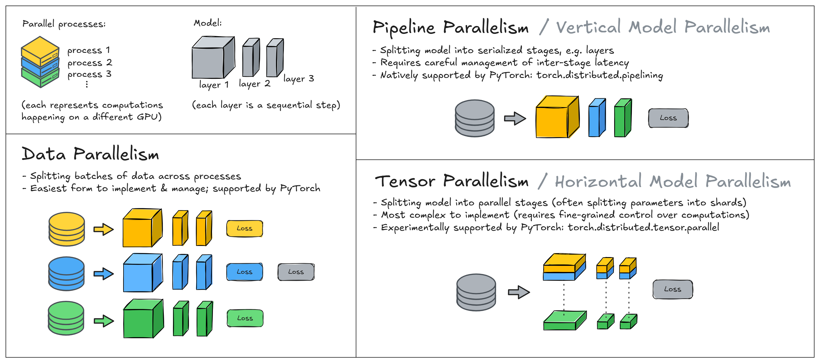
There are 2 main families of distributed training methods: data parallelism and model parallelism. In data parallelism, we split batches of data across different processes, run forward & backward passes on each separately, and accumulate the gradients to update the model parameters. In model parallelism, the model is segmented into different parts that can run concurrently in different nodes, and each one runs on the same data. Model parallelism further splits into horizontal and vertical parallelism depending on whether we're splitting the model up into sequential or parallel parts. Most often horizontal parallelism is called tensor parallelism (because it involves splitting up the weights in a single layer across multiple GPUs, into what we commonly call sharded weights), and vertical parallelism is called pipeline parallelism.

Data & model parallelism are both widely used, and can be more or less appropriate in different circumstances (e.g. some kind of model parallelism is necessary when your model is too large to fit on a single GPU). However it is possible to create hybrid forms of parallelism by combining these; this is especially common when training large models like current SOTA LLMs. In these exercises, we'll focus on just data parallelism, although we'll suggest a few bonus exercises that explore model parallelism.

Summary of exercises

The exercises below will take you through data parallelism. You'll start by learning how to use the basic send and receive functions in PyTorch's distributed training module torch.distributed to transfer tensors between different processes (and different GPUs). Note that you'll need multiple GPUs for these exercises - we've included instructions in a dropdown below.

Once you've done this, you'll use those 2 primitive point-to-point functions to build up some more advanced functions: broadcast (which gets a tensor from one process to all others), gather (which gathers all tensors from different devices to a single device) and all_reduce (which combines both broadcast and gather to make aggregate tensor values across all processes). These functions (all_reduce in particular) are key parts of how distributed computing works.

Lastly, you'll learn how to use these functions to build a distributed training loop, which will be adapted from the ResNetTrainer code from your previous exercises. We also explain how you can use DistributedDataParallel to abstract away these low-level operations, which you might find useful later on (although you will benefit from building these components up from scratch, and understanding how they work under the hood).

Running these exercises

These exercises can't all be run in a notebook or Colab, because distributed training typically requires spawning multiple processes and Jupyter notebooks run in a single interactive process - they're not designed for this kind of use-case.

You have 2 different options:

1. Do everything in a Python file (either # %%-separated cells or execute on selection), but make sure to wrap any execution code in if __name__ == "__main__": blocks. This makes sure that when you launch multiple processes they don't recursively launch their own processes, and they'll only execute the code you want them to.
2. Write your functions in a Python file, then import & run them in a notebook. For example in the example code below, you could define the send_receive function in a Python file, then import this function & pass it into the mp.spawn() call.

In either case, make sure when you run mp.spawn you're passing in the most updated version of your function. This means saving the Python file after you make changes, and also using something like importlib.reload() if you're running the code in a notebook.

IN_COLAB = "google.colab" in sys.modules
assert not IN_COLAB, "Should be doing these exercises in VS Code"

Basic send & receiving

The code below is a simplified example that demonstrates distributed communication between multiple processes.

At the highest level, mp.spawn() launches multiple worker processes, each with a unique rank. For each worker, we create a new Python interpreter (called a "child process") which will execute the function passed to mp.spawn (which in this case is send_receive). The function has to have the type signature fn(rank, *args) where args is the tuple we pass into mp.spawn(). The total number of processes is determined by world_size. Note that this isn't the same as the number of GPUs - in fact, in the code below we've not moved any of our data to GPUs, we're just using the distributed API to sync data across multiple processes. We'll introduce GPUs in the code below this!

We require the environment variables MASTER_ADDR and MASTER_PORT to be set before launching & communicating between processes. The former specifies the IP address or hostname of the machine that will act as the central coordinator (the "master" node) for setting up and managing the distributed environment, while the latter specifies the port number that the master node will use for communication. In our case we're running all our processes from a single node, so all we need is for this to be an unused port on our machine.

Now, breaking down the send_receive function line by line:

• dist.init_process_group initializes each process with a common address and port, and a communication backend. It also gives each process a unique rank, so they know who is sending & receiving data.
• If the function is being run by rank 0, then we create a tensor of zeros and send it using dist.send.
• If the function is being run by rank 1, then we create a tensor of ones and wait to receive a tensor from rank 0 using dist.recv. This will overwrite the data in the original tensor that we created, i.e. so we're just left with a tensor of zeros.
• dist.destroy_process_group() is called at the end of the function to destroy the process group and release resources.

The functions dist.send and dist.recv are the basic primitives for point-to-point communication between processes (we'll look at the primitives for collective communication later on). Each recv for a given source process src will wait until it receives a send from that source to continue, and likewise each send to a given destination process dst will wait until it receives a recv from that process to continue. We call these blocking operations (later on we'll look at non-blocking operations).

WORLD_SIZE = t.cuda.device_count()

os.environ["MASTER_ADDR"] = "localhost"
os.environ["MASTER_PORT"] = "12345"


def send_receive(rank, world_size):
    dist.init_process_group(backend="gloo", rank=rank, world_size=world_size)

    if rank == 0:
        # Send tensor to rank 1
        sending_tensor = t.zeros(1)
        print(f"{rank=}, sending {sending_tensor=}")
        dist.send(tensor=sending_tensor, dst=1)
    elif rank == 1:
        # Receive tensor from rank 0
        received_tensor = t.ones(1)
        print(f"{rank=}, creating {received_tensor=}")
        dist.recv(
            received_tensor, src=0
        )  # this line overwrites the tensor's data with our `sending_tensor`
        print(f"{rank=}, received {received_tensor=}")

    dist.destroy_process_group()


if MAIN:
    world_size = 2  # simulate 2 processes
    mp.spawn(
        send_receive,
        args=(world_size,),
        nprocs=world_size,
        join=True,
    )

rank=0, sending sending_tensor=tensor([0.])
rank=1, creating received_tensor=tensor([1.])
rank=1, received received_tensor=tensor([0.])

Now, let's adapt this toy example to work with our multiple GPUs! You can check how many GPUs you have access to using torch.cuda.device_count().

assert t.cuda.is_available()
assert t.cuda.device_count() > 1, "This example requires at least 2 GPUs per machine"

Before writing our new code, let's first return to the backend argument for dist.init_process_group. There are 3 main backends for distributed training: MPI, GLOO and NCCL. The first two are more general-purpose and support both CPU & GPU tensor communication, while NCCL is a GPU-only protocol optimized specifically for NVIDIA GPUs. It provides better bandwidth and lower latency for GPU-GPU communication, and so we'll be using it for subsequent exercises.

When sending & receiving tensors between GPUs with a NCCL backend, there are 3 important things to remember:

1. Send & received tensors should be of the same datatype.
2. Tensors need to be moved to the GPU before sending or receiving.
3. No two processes should be using the same GPU.

Because of this third point, each process rank will be using the GPU with index rank - hence we'll sometimes refer to the process rank and its corresponding GPU index interchangeably. However it's worth emphasizing that this only applies to our specific data parallelism & NCCL backend example, and so this correspondence doesn't have to exist in general.

The code below is a slightly modified version of the prior code; all we're doing is changing the backend to NCCL & moving the tensors to the appropriate device before sending or receiving.

Note - if at any point during this section you get errors related to the socket, then you can kill the processes by running kill -9 <pid> where <pid> is the process ID. If the process ID isn't given in the error message, you can find it using lsof -i :<port> where <port> is the port number specified in os.environ["MASTER_PORT"] (note you might have to sudo apt-get install lsof before you can run this). If your code is still failing, try changing the port in os.environ["MASTER_PORT"] and running it again.

def send_receive_nccl(rank, world_size):
    dist.init_process_group(backend="nccl", rank=rank, world_size=world_size)

    device = t.device(f"cuda:{rank}")

    if rank == 0:
        # Create a tensor, send it to rank 1
        sending_tensor = t.tensor([rank], device=device)
        print(f"{rank=}, {device=}, sending {sending_tensor=}")
        dist.send(sending_tensor, dst=1)  # Send tensor to CPU before sending
    elif rank == 1:
        # Receive tensor from rank 0 (it needs to be on the CPU before receiving)
        received_tensor = t.tensor([rank], device=device)
        print(f"{rank=}, {device=}, creating {received_tensor=}")
        dist.recv(
            received_tensor, src=0
        )  # this line overwrites the tensor's data with our `sending_tensor`
        print(f"{rank=}, {device=}, received {received_tensor=}")

    dist.destroy_process_group()


if MAIN:
    world_size = 2  # simulate 2 processes
    mp.spawn(
        send_receive_nccl,
        args=(world_size,),
        nprocs=world_size,
        join=True,
    )

rank=1, device=device(type='cuda', index=1), creating received_tensor=tensor([1], device='cuda:1')
rank=0, device=device(type='cuda', index=0), sending sending_tensor=tensor([0], device='cuda:0')
rank=1, device=device(type='cuda', index=1), received received_tensor=tensor([0], device='cuda:1')

Collective communication primitives

We'll now move from basic point-to-point communication to collective communication. This refers to operations that synchronize data across multiple processes, rather than just between a single sender and receiver. There are 3 important kinds of collective communication functions:

• Broadcast: send a tensor from one process to all other processes
• Gather: collect tensors from all processes and concatenates them into a single tensor
• Reduce: like gather, but perform a reduction operation (e.g. sum, mean) rather than concatenation

The latter 2 functions have different variants depending on whether you want the final result to be in just a single destination process or in all of them: for example dist.gather will gather data to a single destination process, while dist.all_gather will make sure every process ends up with all the data.

The functions we're most interested in building are broadcast and all_reduce - the former for making sure all processes have the same initial model parameters, and the latter for aggregating gradients across all processes.

Exercise - implement broadcast

```yaml Difficulty: 🔴🔴🔴⚪⚪ Importance: 🔵🔵🔵⚪⚪

You should spend up to 10-20 minutes on this exercise. ```

Below, you should implement broadcast. If you have tensor $T_i$ on process $i$ for each index, then after running this function you should have $T_s$ on all processes, where $s$ is the source process. If you're confused, you can see exactly what is expected of you by reading the test code in tests.py. Again, remember that you should be running tests either from the command line or in the Python interactive terminal, not in a notebook cell.

def broadcast(tensor: Tensor, rank: int, world_size: int, src: int = 0):
    """
    Broadcast averaged gradients from rank 0 to all other ranks.
    """
    raise NotImplementedError()


if MAIN:
    tests.test_broadcast(broadcast, WORLD_SIZE)

Rank 1 broadcasted tensor: expected 0.0 (from rank 0), got tensor([0.], device='cuda:1')
Rank 0 broadcasted tensor: expected 0.0 (from rank 0), got tensor([0.], device='cuda:0')
Rank 2 broadcasted tensor: expected 0.0 (from rank 0), got tensor([0.], device='cuda:2')
All tests in `test_broadcast` passed!

def broadcast(tensor: Tensor, rank: int, world_size: int, src: int = 0):
    """
    Broadcast averaged gradients from rank 0 to all other ranks.
    """
    if rank == src:
        for other_rank in range(world_size):
            if other_rank != src:
                dist.send(tensor, dst=other_rank)
    else:
        received_tensor = t.zeros_like(tensor)
        dist.recv(received_tensor, src=src)
        tensor.copy_(received_tensor)

Exercise - implement all_reduce

```yaml Difficulty: 🔴🔴🔴⚪⚪ Importance: 🔵🔵🔵⚪⚪

You should spend up to 10-20 minutes on this exercise. ```

You should now implement reduce and all_reduce. The former will aggregate the tensors at some destination process (either sum or mean), and the latter will do the same but then broadcast the result to all processes.

Note, more complicated allreduce algorithms exist than this naive one, and you'll be able to look at some of them in the bonus material.

def reduce(tensor, rank, world_size, dst=0, op: Literal["sum", "mean"] = "sum"):
    """
    Reduces gradients to rank `dst`, so this process contains the sum or mean of all tensors across
    processes.
    """
    raise NotImplementedError()


def all_reduce(tensor, rank, world_size, op: Literal["sum", "mean"] = "sum"):
    """
    Allreduce the tensor across all ranks, using 0 as the initial gathering rank.
    """
    raise NotImplementedError()


if MAIN:
    tests.test_reduce(reduce, WORLD_SIZE)
    tests.test_all_reduce(all_reduce, WORLD_SIZE)

def reduce(tensor, rank, world_size, dst=0, op: Literal["sum", "mean"] = "sum"):
    """
    Reduces gradients to rank dst, so this process contains the sum or mean of all tensors across
    processes.
    """
    if rank != dst:
        dist.send(tensor, dst=dst)
    else:
        for other_rank in range(world_size):
            if other_rank != dst:
                received_tensor = t.zeros_like(tensor)
                dist.recv(received_tensor, src=other_rank)
                tensor += received_tensor
    if op == "mean":
        tensor /= world_size
def all_reduce(tensor, rank, world_size, op: Literal["sum", "mean"] = "sum"):
    """
    Allreduce the tensor across all ranks, using 0 as the initial gathering rank.
    """
    reduce(tensor, rank, world_size, dst=0, op=op)
    broadcast(tensor, rank, world_size, src=0)

Once you've passed these tests, you can run the code below to see how this works for a toy example of model training. In this case our model just has a single parameter and we're performing gradient descent using the squared error between its parameters and the input data as our loss function (in other words we're training the model's parameters to equal the mean of the input data).

The data in the example below is the same as the rank index, i.e. r = 0, 1. For initial parameter x = 2 this gives us errors of (x-r).pow(2) = 4, 2 respectively, and gradients of 2x(x-r) = 8, 4. Averaging these gives us a gradient of 6, so after a single optimization step with learning rate lr=0.1 we get our gradients changing to 2.0 - 0.6 = 1.4.

class SimpleModel(t.nn.Module):
    def __init__(self):
        super(SimpleModel, self).__init__()
        self.param = t.nn.Parameter(t.tensor([2.0]))

    def forward(self, x: Tensor):
        return x - self.param


def run_simple_model(rank, world_size):
    dist.init_process_group(backend="nccl", rank=rank, world_size=world_size)

    device = t.device(f"cuda:{rank}")
    model = SimpleModel().to(device)  # Move the model to the device corresponding to this process
    optimizer = t.optim.SGD(model.parameters(), lr=0.1)

    input = t.tensor([rank], dtype=t.float32, device=device)
    output = model(input)
    loss = output.pow(2).sum()
    loss.backward()  # Each rank has separate gradients at this point

    print(f"Rank {rank}, before all_reduce, grads: {model.param.grad=}")
    all_reduce(model.param.grad, rank, world_size)  # Synchronize gradients
    print(
        f"Rank {rank}, after all_reduce, synced grads (summed over processes): {model.param.grad=}"
    )

    optimizer.step()  # Step with the optimizer (this will update all models the same way)
    print(f"Rank {rank}, new param: {model.param.data}")

    dist.destroy_process_group()


if MAIN:
    world_size = 2
    mp.spawn(
        run_simple_model,
        args=(world_size,),
        nprocs=world_size,
        join=True,
    )

Rank 1, before all_reduce, grads: model.param.grad=tensor([2.], device='cuda:1')
Rank 0, before all_reduce, grads: model.param.grad=tensor([4.], device='cuda:0')
Rank 0, after all_reduce, synced grads (summed over processes): model.param.grad=tensor([6.], device='cuda:0')
Rank 1, after all_reduce, synced grads (summed over processes): model.param.grad=tensor([6.], device='cuda:1')
Rank 0, new param: tensor([1.4000], device='cuda:0')
Rank 1, new param: tensor([1.4000], device='cuda:1')

Full training loop

We'll now use everything we've learned to put together a full training loop! Rather than finetuning it which we've been doing so far, you'll be training your resnet from scratch (although still using the same CIFAR10 dataset). We've given you a function get_untrained_resnet which uses the ResNet34 class from yesterday's solutions, although you're encouraged to replace this function with your implementation if you've completed those exercises.

There are 4 key elements you'll need to change from the non-distributed version of training:

1. Weight broadcasting at initialization
   • For each process you'll need to initialize your model and move it onto the corresponding GPU, but you also want to make sure each process is working with the same model. You do this by broadcasting weights in the __init__ method, e.g. using process 0 as the shared source process.
   • Note - you may find you'll have to brodcast param.data rather than param when you iterate through the model's parameters, because broadcasting only works for tensors not parameters. Parameters are a special class wrapping around and extending standard PyTorch tensors - we'll look at this in more detail tomorrow!
2. Dataloader sampling at each epoch
   • Distributed training works by splitting each batch of data across all the running processes, and so we need to implement this by splitting each batch randomly across our GPUs.
   • Some sample code for this is given below - we recommend you start with this (although you're welcome to play around with some of the parameters here like num_workers and pin_memory).
3. Parameter syncing after each training step
   • After each loss.backward() call but before stepping with the optimizer, you'll need to use all_reduce to sync gradients across each parameter in the model.
   • Just like in the example we gave above, calling all_reduce on param.grad should work, because .grad is a standard PyTorch tensor.
4. Aggregating correct predictions after each evaluation step*
   • We can also split the evaluation step across GPUs - we use all_reduce at the end of the evaluate method to sum the total number of correct predictions across GPUs.
   • This is optional, and often it's not implemented because the evaluation step isn't a bottleneck compared to training, however we've included it in our solutions for completeness.

self.train_sampler = t.utils.data.DistributedSampler(
    self.trainset,
    num_replicas=args.world_size, # we'll divide each batch up into this many random sub-batches
    rank=self.rank, # this determines which sub-batch this process gets
)
self.train_loader = t.utils.data.DataLoader(
    self.trainset,
    self.args.batch_size, # this is the sub-batch size, i.e. the batch size that each GPU gets
    sampler=self.train_sampler, 
    num_workers=2,  # setting this low so as not to risk bottlenecking CPU resources
    pin_memory=True,  # this can improve data transfer speed between CPU and GPU
)
for epoch in range(self.args.epochs):
self.train_sampler.set_epoch(epoch)
for imgs, labels in self.train_loader:
    ...

Exercise - complete DistResNetTrainer

```yaml Difficulty: 🔴🔴🔴🔴🔴 Importance: 🔵🔵🔵⚪⚪

You should spend up to 30-60 minutes on this exercise. If you get stuck on specific bits, you're encouraged to look at the solutions for guidance. ```

We've given you the function dist_train_resnet_from_scratch which you'll be able to pass into mp.spawn just like the examples above, and we've given you a very light template for the DistResNetTrainer class which you should fill in. Your job is just to make the 4 adjustments described above. We recommend not using inheritance for this, because there are lots of minor modifications you'll need to make to the previous code and so you won't be reducing code duplication by very much.

A few last tips before we get started:

• If your code is running slowly, we recommend you also wandb.log the duration of each stage of the training step from the rank 0 process (fwd pass, bwd pass, and all_reduce for parameter syncing), as well as logging the duration of the training & evaluation phases across the epoch. These kinds of logs are generally very helpful for debugging slow code.
• Since running this code won't directly return your model as output, it's good practice to save your model at the end of training using torch.save.
• We recommend you increment examples_seen by the total number of examples across processes, i.e. len(input) * world_size. This will help when you're comparing across different runs with different world sizes (it's convenient for them to have a consistent x-axis).

def get_untrained_resnet(n_classes: int) -> ResNet34:
    """
    Gets untrained resnet using code from part2_cnns.solutions (you can replace this with your
    implementation).
    """
    resnet = ResNet34()
    resnet.out_layers[-1] = Linear(resnet.out_features_per_group[-1], n_classes)
    return resnet


@dataclass
class DistResNetTrainingArgs(WandbResNetFinetuningArgs):
    world_size: int = 1
    wandb_project: str | None = "day3-resnet-dist-training"


class DistResNetTrainer:
    args: DistResNetTrainingArgs

    def __init__(self, args: DistResNetTrainingArgs, rank: int):
        self.args = args
        self.rank = rank
        self.device = t.device(f"cuda:{rank}")

    def pre_training_setup(self):
        raise NotImplementedError()

    def training_step(self, imgs: Tensor, labels: Tensor) -> Tensor:
        raise NotImplementedError()

    @t.inference_mode()
    def evaluate(self) -> float:
        raise NotImplementedError()

    def train(self):
        raise NotImplementedError()


def dist_train_resnet_from_scratch(rank, world_size):
    dist.init_process_group(backend="nccl", rank=rank, world_size=world_size)
    args = DistResNetTrainingArgs(world_size=world_size)
    trainer = DistResNetTrainer(args, rank)
    trainer.train()
    dist.destroy_process_group()


if MAIN:
    world_size = t.cuda.device_count()
    mp.spawn(
        dist_train_resnet_from_scratch,
        args=(world_size,),
        nprocs=world_size,
        join=True,
    )

def get_untrained_resnet(n_classes: int) -> ResNet34:
    """
    Gets untrained resnet using code from part2_cnns.solutions (you can replace this with your
    implementation).
    """
    resnet = ResNet34()
    resnet.out_layers[-1] = Linear(resnet.out_features_per_group[-1], n_classes)
    return resnet
@dataclass
class DistResNetTrainingArgs(WandbResNetFinetuningArgs):
    world_size: int = 1
    wandb_project: str | None = "day3-resnet-dist-training"
class DistResNetTrainer:
    args: DistResNetTrainingArgs
def __init__(self, args: DistResNetTrainingArgs, rank: int):
        self.args = args
        self.rank = rank
        self.device = t.device(f"cuda:{rank}")
def pre_training_setup(self):
        self.model = get_untrained_resnet(self.args.n_classes).to(self.device)
        if self.args.world_size > 1:
            for param in self.model.parameters():
                broadcast(param.data, self.rank, self.args.world_size, src=0)
                # dist.broadcast(param.data, src=0)
self.optimizer = t.optim.AdamW(
            self.model.parameters(), lr=self.args.learning_rate, weight_decay=self.args.weight_decay
        )
self.trainset, self.testset = get_cifar()
        self.train_sampler = self.test_sampler = None
        if self.args.world_size > 1:
            self.train_sampler = DistributedSampler(
                self.trainset, num_replicas=self.args.world_size, rank=self.rank
            )
            self.test_sampler = DistributedSampler(
                self.testset, num_replicas=self.args.world_size, rank=self.rank
            )
        dataloader_shared_kwargs = dict(
            batch_size=self.args.batch_size, num_workers=2, pin_memory=True
        )
        self.train_loader = DataLoader(
            self.trainset, sampler=self.train_sampler, dataloader_shared_kwargs
        )
        self.test_loader = DataLoader(
            self.testset, sampler=self.test_sampler, dataloader_shared_kwargs
        )
        self.examples_seen = 0
if self.rank == 0:
            wandb.init(
                project=self.args.wandb_project,
                name=self.args.wandb_name,
                config=self.args,
            )
def training_step(self, imgs: Tensor, labels: Tensor) -> Tensor:
        t0 = time.time()
# Forward pass
        imgs, labels = imgs.to(self.device), labels.to(self.device)
        logits = self.model(imgs)
        t1 = time.time()
# Backward pass
        loss = F.cross_entropy(logits, labels)
        loss.backward()
        t2 = time.time()
# Gradient sychronization
        if self.args.world_size > 1:
            for param in self.model.parameters():
                all_reduce(param.grad, self.rank, self.args.world_size, op="mean")
                # dist.all_reduce(param.grad, op=dist.ReduceOp.SUM); param.grad /= self.args.world_size
        t3 = time.time()
# Optimizer step, update examples seen & log data
        self.optimizer.step()
        self.optimizer.zero_grad()
        self.examples_seen += imgs.shape[0] * self.args.world_size
        if self.rank == 0:
            wandb.log(
                {
                    "loss": loss.item(),
                    "fwd_time": (t1 - t0),
                    "bwd_time": (t2 - t1),
                    "dist_time": (t3 - t2),
                },
                step=self.examples_seen,
            )
        return loss
@t.inference_mode()
    def evaluate(self) -> float:
        self.model.eval()
        total_correct, total_samples = 0, 0
for imgs, labels in tqdm(self.test_loader, desc="Evaluating", disable=self.rank != 0):
            imgs, labels = imgs.to(self.device), labels.to(self.device)
            logits = self.model(imgs)
            total_correct += (logits.argmax(dim=1) == labels).sum().item()
            total_samples += len(imgs)
# Turn total_correct & total_samples into a tensor, so we can use all_reduce to sum them
        # across processes
        tensor = t.tensor([total_correct, total_samples], device=self.device)
        all_reduce(tensor, self.rank, self.args.world_size, op="sum")
        total_correct, total_samples = tensor.tolist()
accuracy = total_correct / total_samples
        if self.rank == 0:
            wandb.log({"accuracy": accuracy}, step=self.examples_seen)
        return accuracy
def train(self):
        self.pre_training_setup()
accuracy = self.evaluate()  # our evaluate method is the same as parent class
for epoch in range(self.args.epochs):
            t0 = time.time()
if self.args.world_size > 1:
                self.train_sampler.set_epoch(epoch)
                self.test_sampler.set_epoch(epoch)
self.model.train()
pbar = tqdm(self.train_loader, desc="Training", disable=self.rank != 0)
            for imgs, labels in pbar:
                loss = self.training_step(imgs, labels)
                pbar.set_postfix(loss=f"{loss:.3f}", ex_seen=f"{self.examples_seen=:06}")
accuracy = self.evaluate()
if self.rank == 0:
                wandb.log({"epoch_duration": time.time() - t0}, step=self.examples_seen)
                pbar.set_postfix(
                    loss=f"{loss:.3f}",
                    accuracy=f"{accuracy:.3f}",
                    ex_seen=f"{self.examples_seen=:06}",
                )
if self.rank == 0:
            wandb.finish()
            t.save(self.model.state_dict(), f"resnet_{self.rank}.pth")
def dist_train_resnet_from_scratch(rank, world_size):
    dist.init_process_group(backend="nccl", rank=rank, world_size=world_size)
    args = DistResNetTrainingArgs(world_size=world_size)
    trainer = DistResNetTrainer(args, rank)
    trainer.train()
    dist.destroy_process_group()

Bonus - DDP

In practice, the most convenient way to use DDP is to wrap your model in torch.nn.parallel.DistributedDataParallel, which removes the need for explicitly calling broadcast at the start and all_reduce at the end of each training step. When you define a model in this way, it will automatically broadcast its weights to all processes, and the gradients will sync after each loss.backward() call. Here's the example SimpleModel code from above, rewritten to use these features:

from torch.nn.parallel import DistributedDataParallel as DDP


def run(rank: int, world_size: int):
    dist.init_process_group(backend="nccl", rank=rank, world_size=world_size)

    device = t.device(f"cuda:{rank}")
    model = DDP(SimpleModel().to(device), device_ids=[rank])  # Wrap the model with DDP
    optimizer = t.optim.SGD(model.parameters(), lr=0.1)

    input = t.tensor([rank], dtype=t.float32, device=device)
    output = model(input)
    loss = output.pow(2).sum()
    loss.backward()  # DDP handles gradient synchronization

    optimizer.step()
    print(f"Rank {rank}, new param: {model.module.param.data}")

    dist.destroy_process_group()


if MAIN:
    world_size = 2
    mp.spawn(
        run,
        args=(world_size,),
        nprocs=world_size,
        join=True,
    )

Can you use these features to rewrite your ResNet training code? Can you compare it to the code you wrote and see how much faster the built-in DDP version is? Note, you won't be able to separate the time taken for backward passes and gradient synchronization since these happen in the same line, but you can assume that the time taken for the backward pass is approximately unchanged and so any speedup you see is due to the better gradient synchronization.

Bonus - ring operations

Our all reduce operation would scale quite badly when we have a large number of models. It chooses a single process as the source process to receive then send out all data, and so this process risks becoming a bottleneck. One of the most popular alternatives is ring all-reduce. Broadly speaking, ring-based algorithms work by sending data in a cyclic pattern (i.e. worker n sends it to worker n+1 % N where N is the total number of workers). After each sending round, we perform a reduction operation to the data that was just sent. This blog post illustrates the ring all-reduce algorithm for the sum operation.

Can you implement the ring all-reduce algorithm by filling in the function below & passing tests? Once you've implemented it, you can compare the speed of your ring all-reduce vs the all-reduce we implemented earlier - is it faster? Do you expect it to be faster in this particular case?

def ring_all_reduce(tensor: Tensor, rank, world_size, op: Literal["sum", "mean"] = "sum") -> None:
    """
    Ring all_reduce implementation using non-blocking send/recv to avoid deadlock.
    """
    raise NotImplementedError()


if MAIN:
    tests.test_all_reduce(ring_all_reduce)

def ring_all_reduce(tensor: Tensor, rank, world_size, op: Literal["sum", "mean"] = "sum") -> None:
    """
    Ring all_reduce implementation using non-blocking send/recv to avoid deadlock.
    """
    # Clone the tensor as the "send_chunk" for initial accumulation
    send_chunk = tensor.clone()
# Step 1: Reduce-Scatter phase
    for _ in range(world_size - 1):
        # Compute the ranks involved in this round of sending/receiving
        send_to = (rank + 1) % world_size
        recv_from = (rank - 1 + world_size) % world_size
# Prepare a buffer for the received chunk
        recv_chunk = t.zeros_like(send_chunk)
# Non-blocking send and receive
        send_req = dist.isend(send_chunk, dst=send_to)
        recv_req = dist.irecv(recv_chunk, src=recv_from)
        send_req.wait()
        recv_req.wait()
# Accumulate the received chunk into the tensor
        tensor += recv_chunk
# Update send_chunk for the next iteration
        send_chunk = recv_chunk
# Step 2: All-Gather phase
    send_chunk = tensor.clone()
    for _ in range(world_size - 1):
        # Compute the ranks involved in this round of sending/receiving
        send_to = (rank + 1) % world_size
        recv_from = (rank - 1 + world_size) % world_size
# Prepare a buffer for the received chunk
        recv_chunk = t.zeros_like(send_chunk)
# Non-blocking send and receive, and wait for completion
        send_req = dist.isend(send_chunk, dst=send_to)
        recv_req = dist.irecv(recv_chunk, src=recv_from)
        send_req.wait()
        recv_req.wait()
# Update the tensor with received data
        tensor.copy_(recv_chunk)
# Update send_chunk for the next iteration
        send_chunk = recv_chunk
# Step 3: Average the final result
    if op == "mean":
        tensor /= world_size