2️⃣ Weights and Biases

Learning Objectives

• Write modular, extensible code for training models
• Learn what the most important hyperparameters are, and methods for efficiently searching over hyperparameter space
• Learn how to use Weights & Biases for logging your runs
• Adapt your code from yesterday to log training runs to Weights & Biases, and use this service to run hyperparameter sweeps

Next, we'll look at methods for choosing hyperparameters effectively. You'll learn how to use Weights and Biases, a useful tool for hyperparameter search.

The exercises themselves will be based on your ResNet implementations from yesterday, although the principles should carry over to other models you'll build in this course (such as transformers next week).

Note, this page only contains a few exercises, and they're relatively short. You're encouraged to spend some time playing around with Weights and Biases, but you should also spend some more time finetuning your ResNet from yesterday (you might want to finetune ResNet during the morning, and look at today's material in the afternoon - you can discuss this with your partner). You should also spend some time reviewing the last three days of material, to make sure there are no large gaps in your understanding.

Finetuning & feature extraction

We'll start with a brief discussion of the related concepts finetuning and feature extraction. If you've already gone through yesterday's bonus material on feature extraction then you can skip this section.

Finetuning can mean slightly different things in different contexts, but broadly speaking it means using the weights of an already trained network as the starting values for training a new network. Because training networks from scratch is very computationally expensive, this is a common practice in ML.

The specific type of finetuning we'll be doing here is called feature extraction. This is when we freeze most layers of a model except the last few, and perform gradient descent on those. We call this feature extraction because the earlier layers of the model have already learned to identify important features of the data (and these features are also relevant for the new task), so all that we have to do is train a few final layers in the model to extract these features.

Terminology note - sometimes feature extraction and finetuning are defined differently, with finetuning referring to the training of all the weights in a pretrained model (usually with a small or decaying learning rate), and feature extraction referring to the freezing of some layers and training of others. To avoid confusion here, we'll use the term "feature extraction" rather than "finetuning".

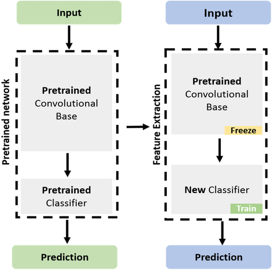
The way we implement feature extraction in PyTorch is by freezing all but the last few layers of our model, meaning gradients don't propagate back through them (and we don't perform gradient descent updates on them) - more on gradient freezing tomorrow! We've used the get_resnet_for_feature_extraction function to do this (the code for this is given to you below so you won't have to write it yourself). This function creates a version of the ResNet34 model, loads in weights from the PyTorch ResNet34 implementation, freezes all layers, and replaces the final linear layer with an unfrozen randomly initialized linear layer with a certain number of output features (in our case 10 because we're doing feature extraction on CIFAR10 - see next section).

CIFAR10

The benchmark we'll be doing feature extraction on is CIFAR10, which consists of 60000 32x32 colour images in 10 different classes (as opposed to the 1000 different classes that ResNet34 was originally trained on). Don't peek at what other people online have done for CIFAR10 (it's a common benchmark), because the point is to develop your own process by which you can figure out how to improve your model. Just reading the results of someone else would prevent you from learning how to get the answers. To get an idea of what's possible: using one V100 and a modified ResNet, one entry in the DAWNBench competition was able to achieve 94% test accuracy in 24 epochs and 76 seconds. 94% is approximately human level performance.

Below is some boilerplate code for downloading and transforming CIFAR10 data (this shouldn't take more than a minute to run the first time). Note, even though CIFAR10 data is 32x32, we'll resize it to 224x224 like we did for ImageNet yesterday, because ResNet expects 224x224 images as input.

def get_cifar() -> tuple[datasets.CIFAR10, datasets.CIFAR10]:
    """Returns CIFAR-10 train and test sets."""
    cifar_trainset = datasets.CIFAR10(
        exercises_dir / "data", train=True, download=True, transform=IMAGENET_TRANSFORM
    )
    cifar_testset = datasets.CIFAR10(
        exercises_dir / "data", train=False, download=True, transform=IMAGENET_TRANSFORM
    )
    return cifar_trainset, cifar_testset


IMAGE_SIZE = 224
IMAGENET_MEAN = [0.485, 0.456, 0.406]
IMAGENET_STD = [0.229, 0.224, 0.225]

IMAGENET_TRANSFORM = transforms.Compose(
    [
        transforms.ToTensor(),
        transforms.Resize((IMAGE_SIZE, IMAGE_SIZE)),
        transforms.Normalize(mean=IMAGENET_MEAN, std=IMAGENET_STD),
    ]
)


cifar_trainset, cifar_testset = get_cifar()

imshow(
    cifar_trainset.data[:15],
    facet_col=0,
    facet_col_wrap=5,
    facet_labels=[cifar_trainset.classes[i] for i in cifar_trainset.targets[:15]],
    title="CIFAR-10 images",
    height=600,
    width=1000,
)

Train function (modular)

First, let's build on the training function we used yesterday. Previously, we just used a single train function which took a dataclass as argument. But this resulted in a very long function with many nested loops and some repeated code. Instead, we'll write our code in the form of a ResNetFinetuner class with multiple methods, each one being responsible for a single part of the training process. This will make our code more modular, and easier to read and debug.

We've given you the ResNetFinetuner class below, as well as a dataclass which contains all the hyperparameters we'll use (again this helps us keep everything organized). You should read this and make sure you understand the role of each method. A brief summary:

• pre_training_setup defines the model, optimizer, dataset, and objects for logging data. Note that it's not good practice to have this logic run in __init__, because it's something we only need to do just before actually training (this structural flexibility will prove useful later, when we introduce weights & biases).
• training_step does a single gradient update step on a single batch of data, and logs & returns the loss.
• evaluate method computes the total accuracy of the model over the validation set, and logs & returns this accuracy. Note use of the torch.inference_mode() decorator, which stops gradients propagating (this is equivalent to using it as a context manager).
• train combines this all: it performs the pre-training setup, then alternates between training & evaluation for some number of epochs. Note that model.train() and model.eval() are called before these stages respectively - for why we have to do this, see yesterday's discussion of BatchNorm.

@dataclass
class ResNetFinetuningArgs:
    n_classes: int = 10
    batch_size: int = 128
    epochs: int = 3
    learning_rate: float = 1e-3
    weight_decay: float = 0.0


class ResNetFinetuner:
    def __init__(self, args: ResNetFinetuningArgs):
        self.args = args

    def pre_training_setup(self):
        self.model = get_resnet_for_feature_extraction(self.args.n_classes).to(device)
        self.optimizer = AdamW(
            self.model.out_layers[-1].parameters(),
            lr=self.args.learning_rate,
            weight_decay=self.args.weight_decay,
        )
        self.trainset, self.testset = get_cifar()
        self.train_loader = DataLoader(self.trainset, batch_size=self.args.batch_size, shuffle=True)
        self.test_loader = DataLoader(self.testset, batch_size=self.args.batch_size, shuffle=False)
        self.logged_variables = {"loss": [], "accuracy": []}
        self.examples_seen = 0

    def training_step(
        self,
        imgs: Float[Tensor, "batch channels height width"],
        labels: Int[Tensor, "batch"],
    ) -> Float[Tensor, ""]:
        """Perform a gradient update step on a single batch of data."""
        imgs, labels = imgs.to(device), labels.to(device)

        logits = self.model(imgs)
        loss = F.cross_entropy(logits, labels)
        loss.backward()
        self.optimizer.step()
        self.optimizer.zero_grad()

        self.examples_seen += imgs.shape[0]
        self.logged_variables["loss"].append(loss.item())
        return loss

    @t.inference_mode()
    def evaluate(self) -> float:
        """Evaluate the model on the test set and return the accuracy."""
        self.model.eval()
        total_correct, total_samples = 0, 0

        for imgs, labels in tqdm(self.test_loader, desc="Evaluating"):
            imgs, labels = imgs.to(device), labels.to(device)
            logits = self.model(imgs)
            total_correct += (logits.argmax(dim=1) == labels).sum().item()
            total_samples += len(imgs)

        accuracy = total_correct / total_samples
        self.logged_variables["accuracy"].append(accuracy)
        return accuracy

    def train(self) -> dict[str, list[float]]:
        self.pre_training_setup()

        accuracy = self.evaluate()

        for epoch in range(self.args.epochs):
            self.model.train()

            pbar = tqdm(self.train_loader, desc="Training")
            for imgs, labels in pbar:
                loss = self.training_step(imgs, labels)
                pbar.set_postfix(loss=f"{loss:.3f}", ex_seen=f"{self.examples_seen:06}")

            accuracy = self.evaluate()
            pbar.set_postfix(
                loss=f"{loss:.3f}", accuracy=f"{accuracy:.2f}", ex_seen=f"{self.examples_seen:06}"
            )

        return self.logged_variables

With this class, we can perform feature extraction on our model as follows:

args = ResNetFinetuningArgs()
trainer = ResNetFinetuner(args)
logged_variables = trainer.train()


line(
    y=[logged_variables["loss"][: 391 * 3 + 1], logged_variables["accuracy"][:4]],
    x_max=len(logged_variables["loss"][: 391 * 3 + 1] * args.batch_size),
    yaxis2_range=[0, 1],
    use_secondary_yaxis=True,
    labels={"x": "Examples seen", "y1": "Cross entropy loss", "y2": "Test Accuracy"},
    title="Feature extraction with ResNet34",
    width=800,
)

Files already downloaded and verified
Files already downloaded and verified
Evaluating: 100%|██████████| 79/79 [00:23<00:00,  3.30it/s]
Training: 100%|██████████| 391/391 [02:06<00:00,  3.09it/s, ex_seen=050000, loss=0.744]
Evaluating: 100%|██████████| 79/79 [00:23<00:00,  3.39it/s]
Training: 100%|██████████| 391/391 [02:05<00:00,  3.10it/s, ex_seen=100000, loss=0.731]
Evaluating: 100%|██████████| 79/79 [00:22<00:00,  3.44it/s]
Training: 100%|██████████| 391/391 [02:05<00:00,  3.13it/s, ex_seen=150000, loss=0.584]
Evaluating: 100%|██████████| 79/79 [00:22<00:00,  3.44it/s]

Let's see how well our ResNet performs on the first few inputs!

def test_resnet_on_random_input(model: ResNet34, n_inputs: int = 3, seed: int | None = 42):
    if seed is not None:
        np.random.seed(seed)
    indices = np.random.choice(len(cifar_trainset), n_inputs).tolist()
    classes = [cifar_trainset.classes[cifar_trainset.targets[i]] for i in indices]
    imgs = cifar_trainset.data[indices]
    device = next(model.parameters()).device
    with t.inference_mode():
        x = t.stack(list(map(IMAGENET_TRANSFORM, imgs)))
        logits: Tensor = model(x.to(device))
    probs = logits.softmax(-1)
    if probs.ndim == 1:
        probs = probs.unsqueeze(0)
    for img, label, prob in zip(imgs, classes, probs):
        display(HTML(f"<h2>Classification probabilities (true class = {label})</h2>"))
        imshow(img, width=200, height=200, margin=0, xaxis_visible=False, yaxis_visible=False)
        bar(
            prob,
            x=cifar_trainset.classes,
            width=600,
            height=400,
            text_auto=".2f",
            labels={"x": "Class", "y": "Prob"},
        )


test_resnet_on_random_input(trainer.model)

What is Weights and Biases?

Weights and Biases is a cloud service that allows you to log data from experiments. Your logged data is shown in graphs during training, and you can easily compare logs across different runs. It also allows you to run sweeps, where you can specifiy a distribution over hyperparameters and then start a sequence of test runs which use hyperparameters sampled from this distribution.

Before you run any of the code below, you should visit the Weights and Biases homepage, and create your own account.

We'll be able to keep the same structure of training loop when using weights and biases, we'll just have to add a few functions. The key functions to know are:

wandb.init

This initialises a training run. It should be called once, at the start of your training loop.

A few important arguments are:

• project - the name of the project where you're sending the new run. For example, this could be 'day3-resnet' for us. You can have many different runs in each project.
• name - a display name for this run. By default, if this isn't supplied, wandb generates a random 2-word name for you (e.g. gentle-sunflower-42).
• config - a dictionary containing hyperparameters for this run. If you pass this dictionary, then you can compare different runs' hyperparameters & results in a single table. Alternatively, you can pass a dataclass.

wandb.watch

This function tells wandb to watch a model - this means that it will log the gradients and parameters of the model during training. We'll call this function once, after we've created our model. The 3 most important arguments are:

• models - a module or list of modules (e.g. in our case we might just want to log the weights of the final linear layer, because the others aren't being trained)
• log - determines what gets tracked, possible values are 'gradients' (default), 'parameters' or 'all'
• log_freq - the number of batches between each logging step (default is 1000)

Why do we log parameters and gradients? Mainly this is helpful for debugging, because it helps us identify problems like exploding or vanishing gradients, dead ReLUs, etc.

wandb.log

For logging metrics to the wandb dashboard. This is used as wandb.log(data, step), where step is an integer (the x-axis on your metric plots) and data is a dictionary of metrics (i.e. the keys are metric names, and the values are metric values).

wandb.finish

This function should be called at the end of your training loop. It finishes the run, and saves the results to the cloud.

If a run terminates early (either because of an error or because you manually terminated it), remember to still run wandb.finish() - it will speed things up when you start a new run (otherwise you have to wait for the previous run to be terminated & uploaded).

Exercise - rewrite training loop with wandb

```yaml Difficulty: 🔴🔴⚪⚪⚪ Importance: 🔵🔵🔵🔵⚪

You should spend up to 10-25 minutes on this exercise. ```

You should now take the training loop from above (i.e. the ResNetTrainer class) and rewrite it to use the four wandb functions above (in place of the logged_variables dictionary, which you can now remove). This will require:

• Initializing your run
  • Your new pre_training_setup method should call wandb.watch and wandb.init as well as all the stuff it previously did
  • For wandb.init, you can use the project & name arguments from your new dataclass (see below)
  • For wandb.watch, be careful of the log_freq value - you want to make sure you're logging more than once per epoch
• Logging variables to wandb during your run
  • i.e. replace updating of self.logged_variables with calls to wandb.log
  • We recommend tracking self.examples_seen and passing this as the step argument to your logging calls, this way it's easier to compare across different runs with e.g. different batch sizes (more on this later)
• Finishing the run
  • i.e. calling wandb.finish at the end of your training loop

This is all you need to do to get wandb working, so the vast majority of the code you write below will be copied and pasted from the previous ResNetFinetuner class. We've given you a template for this below, along with a new dataclass. Both the dataclass and the trainer class use inheritance to remove code duplication (e.g. because we don't need to rewrite our __init__ method, it'll be the same as for ResNetFinetuner).

Note, we generally recommend keeping progress bars in wandb because they update slightly faster and can give you a better sense of whether something is going wrong in training.

@dataclass
class WandbResNetFinetuningArgs(ResNetFinetuningArgs):
    """Contains new params for use in wandb.init, as well as all the ResNetFinetuningArgs params."""

    wandb_project: str | None = "day3-resnet"
    wandb_name: str | None = None


class WandbResNetFinetuner(ResNetFinetuner):
    args: WandbResNetFinetuningArgs  # adding this line helps with typechecker!
    examples_seen: int = 0  # tracking examples seen (used as step for wandb)

    def pre_training_setup(self):
        """Initializes the wandb run using `wandb.init` and `wandb.watch`."""
        super().pre_training_setup()
        raise NotImplementedError()

    def training_step(
        self,
        imgs: Float[Tensor, "batch channels height width"],
        labels: Int[Tensor, "batch"],
    ) -> Float[Tensor, ""]:
        """Equivalent to ResNetFinetuner.training_step, but logging the loss to wandb."""
        raise NotImplementedError()

    @t.inference_mode()
    def evaluate(self) -> float:
        """Equivalent to ResNetFinetuner.evaluate, but logging the accuracy to wandb."""
        raise NotImplementedError()

    def train(self) -> None:
        """Equivalent to ResNetFinetuner.train, but with wandb integration."""
        self.pre_training_setup()
        raise NotImplementedError()


args = WandbResNetFinetuningArgs()
trainer = WandbResNetFinetuner(args)
trainer.train()

@dataclass
class WandbResNetFinetuningArgs(ResNetFinetuningArgs):
    """Contains new params for use in wandb.init, as well as all the ResNetFinetuningArgs params."""
wandb_project: str | None = "day3-resnet"
    wandb_name: str | None = None
class WandbResNetFinetuner(ResNetFinetuner):
    args: WandbResNetFinetuningArgs  # adding this line helps with typechecker!
    examples_seen: int = 0  # tracking examples seen (used as step for wandb)
def pre_training_setup(self):
        """Initializes the wandb run using wandb.init and wandb.watch."""
        super().pre_training_setup()
        wandb.init(project=self.args.wandb_project, name=self.args.wandb_name, config=self.args)
        wandb.watch(self.model.out_layers[-1], log="all", log_freq=50)
        self.examples_seen = 0
def training_step(
        self,
        imgs: Float[Tensor, "batch channels height width"],
        labels: Int[Tensor, "batch"],
    ) -> Float[Tensor, ""]:
        """Equivalent to ResNetFinetuner.training_step, but logging the loss to wandb."""
        imgs, labels = imgs.to(device), labels.to(device)
logits = self.model(imgs)
        loss = F.cross_entropy(logits, labels)
        loss.backward()
        self.optimizer.step()
        self.optimizer.zero_grad()
self.examples_seen += imgs.shape[0]
        wandb.log({"loss": loss.item()}, step=self.examples_seen)
        return loss
@t.inference_mode()
    def evaluate(self) -> float:
        """Equivalent to ResNetFinetuner.evaluate, but logging the accuracy to wandb."""
        self.model.eval()
        total_correct, total_samples = 0, 0
for imgs, labels in tqdm(self.test_loader, desc="Evaluating"):
            imgs, labels = imgs.to(device), labels.to(device)
            logits = self.model(imgs)
            total_correct += (logits.argmax(dim=1) == labels).sum().item()
            total_samples += len(imgs)
accuracy = total_correct / total_samples
        wandb.log({"accuracy": accuracy}, step=self.examples_seen)
        return accuracy
def train(self) -> None:
        """Equivalent to ResNetFinetuner.train, but with wandb integration."""
        self.pre_training_setup()
        accuracy = self.evaluate()
for epoch in range(self.args.epochs):
            self.model.train()
pbar = tqdm(self.train_loader, desc="Training")
            for imgs, labels in pbar:
                loss = self.training_step(imgs, labels)
                pbar.set_postfix(loss=f"{loss:.3f}", ex_seen=f"{self.examples_seen=:06}")
accuracy = self.evaluate()
            pbar.set_postfix(
                loss=f"{loss:.3f}", accuracy=f"{accuracy:.2f}", ex_seen=f"{self.examples_seen=:06}"
            )
wandb.finish()

When you run the code for the first time, you'll have to login to Weights and Biases, and paste an API key into VSCode. After this is done, your Weights and Biases training run will start. It'll give you a lot of output text, one line of which will look like:

View run at https://wandb.ai/<USERNAME>/<PROJECT-NAME>/runs/<RUN-NAME>

which you can click on to visit the run page.

A nice thing about using Weights and Biases is that you don't need to worry about generating your own plots, that will all be done for you when you visit the page.

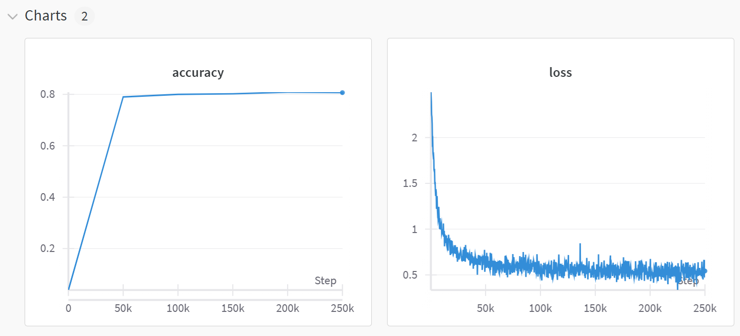
Run & project pages

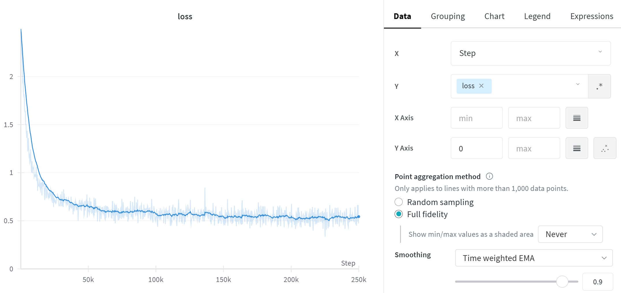
The page you visit will show you a plot of all the variables you've logged, among other things. You can do many things with these plots (e.g. click on the "edit" icon for your train_loss plot, and apply smoothing & change axis bounds to get a better picture of your loss curve).

The charts are a useful feature of the run page that gets opened when you click on the run page link, but they're not the only feature. You can also navigate to the project page (click on the option to the right of Projects on the bar at the top of the Wandb page), and see superimposed plots of all the runs in this project. You can also click on the Table icon on the left hand sidebar to see a table of all the runs in this project, which contains useful information (e.g. runtime, the most recent values of any logged variables, etc). However, comparing runs like this becomes especially useful when we start doing hyperparameter search.

You can also look at the system tab to inspect things like GPU utilization - this is a good way of checking whether you're saturating your GPU or whether you can afford to increase your batch size more. This tab will be especially useful in the next section, when we move onto distributed training.

Some training heuristics

One important skill which every aspiring ML researcher should develop is the ability to play around with hyperparameters and improve a model's training. At times this is more of an art than a science, because frequently rules and heuristics which work most of the time will break down in certain special cases. For example, a common heuristic for number of workers in a DataLoader is to set them to be 4 times the number of GPUs you have available (see later sections on distributed computing for more on this). However, setting these values too high can lead to issues where your CPU is bottlenecked by the workers and your epochs take a long time to start - it took me a long time to realize this was happening when I was initially writing these exercises!

Sweeping over hyperparameters (which we'll cover shortly) can help remove some of the difficulty here, because you can use sweep methods that guide you towards an optimal set of hyperparameter choices rather than having to manually pick your own. However, here are a few heuristics that you might find useful in a variety of situations:

• Setting batch size
  • Generally you should aim to saturate your GPU with data - this means choosing a batch size that's as large as possible without causing memory errors
    • You should generally aim for over 70% utilization of your GPU
  • Note, this means you should generally try for a larger batch size in your testloader than your trainloader (because evaluation is done without gradients, and so a smaller memory constraint)
    • A good starting point is 4x the size, but this will vary between models
• Choosing a learning rate
  • Inspecting loss curves can be a good way of evaluating our learning rate
    • If loss is decreasing very slowly & monotonically then this is a sign you should increase the learning rate, whereas very large loss spikes are a sign that you should decrease it
  • A common strategy is warmup, i.e. having a smaller learning rate for a short period of time at the start of training - we'll do this a lot in later material
  • Jeremy Jordan has a good blog post on learning rates
• Balancing learning rate and batch size
  • For standard optimizers like SGD, it's a good idea to scale the learning rate inversely to the batch size - this way the variance of each parameter step remains the same
  • However for adaptive optimizers such as Adam (where the size of parameter updates automatically adjusts based on the first and second moments of our gradients), this isn't as necessary
    • This is why we generally start with default parameters for Adam, and then adjust from there
• Misc. advice
  • If you're training a larger model, it's sometimes a good idea to start with a smaller version of that same model. Good hyperparameters tend to transfer if the architecture & data is the same; the main difference is the larger model may require more regularization to prevent overfitting.
  • Bad hyperparameters are usually clearly worse by the end of the first 1-2 epochs. You can manually abort runs that don't look promising (or do it automatically - see discussion of Hyperband in wandb sweeps at the end of this section)
  • Overfitting at the start is better than underfitting, because it means your model is capable of learning and has enough capacity

Hyperparameter search

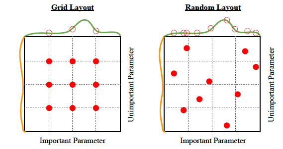
One way to search for good hyperparameters is to choose a set of values for each hyperparameter, and then search all combinations of those specific values. This is called grid search. The values don't need to be evenly spaced and you can incorporate any knowledge you have about plausible values from similar problems to choose the set of values. Searching the product of sets takes exponential time, so is really only feasible if there are a small number of hyperparameters. I would recommend forgetting about grid search if you have more than 3 hyperparameters, which in deep learning is "always".

A much better idea is for each hyperparameter, decide on a sampling distribution and then on each trial just sample a random value from that distribution. This is called random search and back in 2012, you could get a publication for this. The diagram below shows the main reason that random search outperforms grid search. Empirically, some hyperparameters matter more than others, and random search benefits from having tried more distinct values in the important dimensions, increasing the chances of finding a "peak" between the grid points.

It's worth noting that both of these searches are vastly less efficient than gradient descent at finding optima - imagine if you could only train neural networks by randomly initializing them and checking the loss! Either of these search methods without a dose of human (or eventually AI) judgement is just a great way to turn electricity into a bunch of models that don't perform very well.

Running hyperparameter sweeps with wandb

Now we've come to one of the most impressive features of wandb - being able to perform hyperparameter sweeps. We do this by defining a sweep_config dict which tells us how our hyperparameters will be randomly sampled, then we write a train function which takes no arguments and launches a training run with our modified hyperparameters. Lastly we use wandb.sweep and wandb.agent to run our sweep. We'll go through each step of this below.

Sweep config syntax

The basic syntax for a sweep config looks like this:

sweep_config = dict(
    method = method, # can be "grid", "random" or "bayes"
    metric = dict(
        name = metric_name, # name of the metric you're optimising (should be a numeric type logged in `wandb.log`)
        goal = goal, # either "maximize" or "minimize"
    )),
    parameters = dict(
        param_1 = dict(...),
        param_2 = dict(...),
        ...
    ),
)

The method argument determines how we perform search: grid is over all combinations, random independently samples each hyperparameter, and bayes uses Bayesian optimization to sample hyperparameters. The metric dict determines what logged variable we're optimizing, and in what direction. Lastly, parameters is a list of parameters we're varying, with each dictionary describing how we want that parameter to be sampled. Possible ways to specify distributions include:

parameters = dict(
    param_1 = dict(values = [...]), # uniformly sample from list of values
    param_2 = dict(values = [...], probabilities = [...]), # sample from list with given probabilities
    param_3 = dict(min = ..., max = ...), # uniform distribution over [min, max), can either be ints or floats
    param_4 = dict(min = ..., max = ..., distribution = "log_uniform_values"), # use log-uniform distribution instead
)

Note on log uniform distribution - this essentially means we return value s.t. log(value) is uniformly distributed between log(min) and log(max). It can be a useful way to sample hyperparameters which take values in a very large range.

You can read more about the syntax here, but the examples we've given you above should be enough to complete the rest of these exercises.

wandb sweep sweep_config.yaml
wandb agent <SWEEP_ID>

program: train.py
method: random
metric:
    name: test_accuracy
    goal: maximize

Exercise - define a sweep config & update args

```yaml Difficulty: 🔴🔴⚪⚪⚪ Importance: 🔵🔵🔵⚪⚪

You should spend up to 10-20 minutes on this exercise. Learning how to use wandb for sweeps is very useful, so make sure you understand all parts of this code. ```

Using the syntax discussed above, you should define a dictionary sweep_config which has the following rules for hyperparameter sweeps:

• Hyperparameters are chosen randomly, according to the distributions given in the dictionary
• Your goal is to maximize the accuracy metric
• The hyperparameters you vary are:
  • Learning rate - a log-uniform distribution between 1e-4 and 1e-1
  • Batch size - sampled uniformly from (32, 64, 128, 256)
  • Weight decay - with 50% probability set to 0, and with 50% probability log-uniform between 1e-4 and 1e-2

You should also fill in the update_args function, which returns a modified version of args based on the hyperparameters sampled by the sweep. In other words, it should take an args object and a dictionary of sampled parameters that might look something like {"lr": 0.001, "batch_size": 64, ...}, and return a new args object with these fields modified.

# YOUR CODE HERE - fill `sweep_config` so it has the requested behaviour
sweep_config = dict(
    method = ...,
    metric = ...,
    parameters = ...,
)


def update_args(
    args: WandbResNetFinetuningArgs, sampled_parameters: dict
) -> WandbResNetFinetuningArgs:
    """
    Returns a new args object with modified values. The dictionary `sampled_parameters` will have
    the same keys as your `sweep_config["parameters"]` dict, and values equal to the sampled values
    of those hyperparameters.
    """
    assert set(sampled_parameters.keys()) == set(sweep_config["parameters"].keys())

    # YOUR CODE HERE - update `args` based on `sampled_parameters`
    raise NotImplementedError()


tests.test_sweep_config(sweep_config)
tests.test_update_args(update_args, sweep_config)

sweep_config = dict(
    method="random",
    metric=dict(name="accuracy", goal="maximize"),
    parameters=dict(
        learning_rate=dict(min=1e-4, max=1e-1, distribution="log_uniform_values"),
        batch_size=dict(values=[32, 64, 128, 256]),
        weight_decay=dict(min=1e-4, max=1e-2, distribution="log_uniform_values"),
        weight_decay_bool=dict(values=[True, False]),
    ),
)
def update_args(args: WandbResNetFinetuningArgs, sampled_parameters: dict) -> WandbResNetFinetuningArgs:
    assert set(sampled_parameters.keys()) == set(sweep_config["parameters"].keys())
args.learning_rate = sampled_parameters["learning_rate"]
    args.batch_size = sampled_parameters["batch_size"]
    args.weight_decay = sampled_parameters["weight_decay"] if sampled_parameters["weight_decay_bool"] else 0.0
    return args

def update_args(args: WandbResNetFinetuningArgs, sampled_parameters: dict) -> WandbResNetFinetuningArgs:
    assert set(sampled_parameters.keys()) == set(sweep_config["parameters"].keys())
sampled_parameters["weight_decay"] *= float(sampled_parameters.pop("weight_decay_bool"))
    return replace(args, **sampled_parameters)

Now we've done this, we'll define a train function that takes no arguments and launches a training run with our modified hyperparameters. This is done in the following way:

• The train function calls wandb.init
• Our sampled hyperparameters are now available in wandb.config, so we use this object to update args
• We then launch a training run based on these new hyperparameters

The line sweep_id = wandb.sweep(...) initializes a hyperparameter sweep (giving it an ID) and the line wandb.agent(...) starts an agent that runs the training script train 3 times, with different randomly sampled sets of hyperparameters each time.

Note that we pass reinit=False into our wandb.init call - this is so we ignore the second wandb.init call that takes place in our pretraining setup when we run trainer.train() (so we can avoid the hassle of having to rewrite this method to remove that line).

def train():
    # Define args & initialize wandb
    args = WandbResNetFinetuningArgs()
    wandb.init(project=args.wandb_project, name=args.wandb_name, reinit=False)

    # After initializing wandb, we can update args using `wandb.config`
    args = update_args(args, dict(wandb.config))

    # Train the model with these new hyperparameters (the second `wandb.init` call will be ignored)
    trainer = WandbResNetFinetuner(args)
    trainer.train()


sweep_id = wandb.sweep(sweep=sweep_config, project="day3-resnet-sweep")
wandb.agent(sweep_id=sweep_id, function=train, count=3)
wandb.finish()

When you run this code, you should click on the link which looks like:

View sweep at https://wandb.ai/<USERNAME>/<PROJECT-NAME>/sweeps/<SWEEP-NAME>

This link will bring you to a page comparing each of your sweeps. You'll be able to see overlaid graphs of each of their training loss and test accuracy, as well as a bunch of other cool things like:

• Bar charts of the importance (and correlation) of each hyperparameter wrt the target metric. Note that only looking at the correlation could be misleading - something can have a correlation of 1, but still have a very small effect on the metric.
• A parallel coordinates plot, which summarises the relationship between the hyperparameters in your config and the model metric you're optimising.

What can you infer from these results? Are there any hyperparameters which are especially correlated / anticorrelated with the target metric? Are there any results which suggest the model is being undertrained?

You might also want to play around with Bayesian hyperparameter search, if you get the time! Note that wandb sweeps also offer early termination of runs that don't look promising, based on the Hyperband algorithm.

To conclude - wandb is an incredibly useful tool when training models, and you should find yourself using it a fair amount throughout this program. You can always return to this page of exercises if you forget how any part of it works!